Genomics Is Not NLP: A Field Guide for ML Scientists
Published:
Before diving into a discussion of genomics and natural language processing (NLP), we should review a basic primer of molecular biology. For the biologists out there, forgive me for making some oversimplifications. This field is much richer than can be fit in one paragraph! And for the computer scientists out there, there really is more to biology than dissecting frogs and annotating oversaturated printouts of the endoplasmic reticulum.
Molecular biology primer
DNA is the “blueprint” of the human body that holds our genetic code. Every cell in a specific organism possesses identical DNA (barring mutations that accumulate over a person‘s life); it is regulation of this DNA that leads to differences between cell types (eg neuron vs. liver cell). DNA is a large molecule comprised of nucleotides — small chemical subunits that can be abstracted as “letters”. These four nucleotides are adenine (A), cytosine (C), guanine (G), and thymine (T). DNA is packaged into chromosomes. Humans have 46 chromosomes and are diploid — our chromosomes come in pairs, where we inherit half of our chromosomes from our mom and half from our dad. The chromosomes are numbered 1-22 (autosomes — descending order of length) and X/Y (sex chromosomes). The human genome contains ~3.2 billion nucleotides in total. The central dogma of molecular biology describes the fundamental role of DNA: DNA is transcribed into messenger RNA (mRNA), a form of ribonucleic acid (RNA), and mRNA is translated into protein. Only ~1–2% of DNA encodes mRNA; the rest of DNA is involved in regulation of gene expression, transcription into non-coding RNA, structural roles (such as centromeres and telomeres), has uncharacterized function, or may serve no function at all. mRNA is also comprised of nucleotides like DNA, and is grouped into triplets called codons during translation, where each codon encodes an amino acid. Amino acids are the subunit of proteins. There are 20 amino acids (the memorization of which is a rite of passage for every biochemistry student), each characterized by different chemical structures and properties (e.g., polarity, acidity, size, disulfide-bond potential, phosphorylation potential). As there are \(4^{3} = 64\) possible nucleotide combinations in a codon, the existence of only 20 amino acids implies that the genetic code is degenerate: 1-4 codons will encode the same amino acid. Proteins do the work of the cell — they catalyze reactions, communicate signals, transport molecules, build structures, and much more. Effectively, DNA is relevant only insofar that it encodes mRNA, which itself encodes protein — DNA molecules themselves serve essentially no role in the human body outside of this function.
DNA and NLP similarities and differences
At first glance, genomics looks like a direct analog to natural language processing. And in some respects, it is. Both the English language and the genetic code share a small finite alphabet — English has 26 letters, and DNA has four nucleotides (ACGT). Both have an exponentially large number of units that can be formed by unique permutations of this alphabet — English groups letters into words, and DNA groups nucleotides into genes. The two vocabulary sizes are comparable — there are ~20,000 words in the English language and ~20,000 genes encoded in the human body.
But there are also some crucial differences that must be addressed. For instance, English words are often within a narrow length range of 2 to 10 characters. Genes, however, range anywhere between 1,000 to 1,000,000 nucleotides. Changing an English sentence with even a single letter substitution is guaranteed to change the meaning of a sentence, as the similarity in meaning between words holds minimal correlation with similarity in structure. With DNA, some base substitutions are completely invisible, some have modest effects on outcome, and some are catastrophic. Mutations outside gene-coding regions nearly always have no effect. Mutations within gene-coding regions generally only have an effect if they cause a change in amino acid, and especially if they significantly change the chemical properties of the amino acid. Mutations are significant when they result in a change in protein folding structure, which can lead to protein instability or loss of ligand specificity.
DNA and English text also have different numbers of hierarchical groupings. As discussed earlier, nucleotides can be thought of as analogous to letters, and genes can be thought of as analogous to words. Carrying forward this analogy, each chromosome or entire human genome could be thought of as analogous to a document. However, there is no analogue to a “sentence” for DNA. Each “document” would simply read as a list of words used exactly one time, likely ordered based on their position in the genome — an order that has little functional significance. Or, perhaps, different conventions can be applied to DNA. For instance, an alternative representation would be to represent DNA codons as letters, rather than individual nucleotides, which would create a 64 character alphabet rather than a four character alphabet. This would pose its own challenges, however, such as the degeneracy of the DNA code (up to four codons can encode the same amino acid, with the last nucleotide often being flexible) and the questionable relevance of codon-tokenization in non-coding regions (where transcription does not occur). Or, alternatively yet again, if we stick with nucleotides as letters, then these codons or other k-mers (subsequences of length k) could represent words, and genes could represent sentences. But this still runs into the problem of high “sentence” similarity and “document” structure.
Any two English sentences or documents will contain vastly different structure. Some documents might be one sentence, while others might be hundreds of pages long. The lengths of sentences and vocabulary used can vary widely. For text classification, such as sentiment analysis, the entire body of text must be analyzed, as each portion can contribute to the meaning of the text as a whole. In contrast, DNA has a highly consistent structure between individuals. Any two individuals are ~99.9% identical. Of the ~3.2 billion nucleotides in the human genome, only ~10 million nucleotides have substantial (common) variation across the human population1. This shallow diversity is due to a population bottleneck approximately 50,000 years ago which restricted our genetic ancestors to approximately 10,000 individuals. Most of these variants have a most common form, which can be collected into what is called a reference genome1. In addition to these ~10 million sites of possible variation, each person has ~70 de novo mutations that are specific to them3, and any given cell may accumulate up to several thousand somatic mutations over the person’s life4. This means that any artificial intelligence (AI) model that ingests the entire 3.2 billion nucleotide sequence is exerting a lot of unnecessary energy, as most sites are essentially guaranteed to match the reference genome. There are benefits to working with raw DNA sequences as well. The simplicity of the input data, the direct analog to natural language, and the ability to maintain the full context of DNA that is especially relevant for tasks such as mutation effect prediction. But this trade-off is unique to genomics data and should be intentionally considered by the machine learning practitioner.
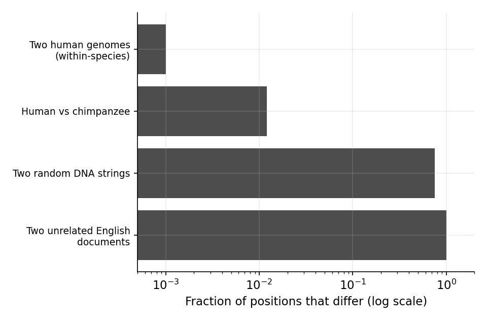
Figure 1: Two members of the human species are near-duplicates. The fraction of positions that differ between two sequences, on a log scale: two humans differ at only ~\(10^{-3}\) of positions and human versus chimpanzee at ~\(10^{-2}\), whereas two random DNA strings differ at \(0.75\) and two unrelated English documents at essentially every position. The within-species genomic “corpus” is roughly a thousandfold more redundant than text.
Sources of genomic data
Genomics data can come from multiple sources. These include whole genome sequencing (WGS; sequencing the entire genome), whole exome sequencing (WES; sequencing only the gene-encoding regions of the genome), bulk RNA-sequencing (bulk RNA-seq; sequencing all expressed RNA), and single-cell RNA sequencing (scRNA-seq; sequencing RNA at single-cell resolution). These sequencing machines have ~99–99.9% per-base accuracy. When only mildly confident about the detected nucleotide, the machine may report a lowercase letter. When entirely unconfident, the machine may report an “N”. How to handle these additional characters is a design decision in any tokenizer.
The protocol to sequence genomic data depends on the assay and technology, but they all share the isolation of genetic material, decomposition into small regions generally between 75-150 nucleotides (reads), amplification by polymerase chain reaction (PCR), and sequence readout. The reads (FASTQ file) are usually mapped to the reference genome (FASTA file) to produce a genome alignment (BAM, or Binary Alignment Map, file). For DNA, the variants can be extracted in a VCF (Variant Call Format) file. For RNA data, the count of each gene can be stored in a count matrix, where each row represents a sample (bulk RNA-seq) or cell (single-cell RNA-seq), and each column represents a gene.
DNA, RNA, and protein
I mentioned earlier that proteins are the real molecule of interest in the human body, so why do we measure RNA at all rather than measuring protein directly? One of the main reasons is that protein sequencing technology has simply lagged behind nucleotide sequencing technology in cost. The underlying assumption is that RNA levels correlate strongly with protein levels, so the former can be used as a proxy for the latter. However, this may be a stronger assumption than most would like to believe. Across many careful studies, the correlation between a gene’s mRNA level and its protein level is moderate at best — typically a Spearman \(\rho\) in the 0.4-0.6 range, and lower still when you look at changes over time rather than steady-state across genes. Schwanhäusser and colleagues found mRNA explained well under half the variance in protein abundance5; Vogel and Marcotte, Liu, Beyer and Aebersold, and Buccitelli and Selbach all converge on the same message — translation rates, protein half-lives, and post-translational regulation drive a large share of protein levels that mRNA simply does not see6–8. Edfors and colleagues showed the relationship is gene-specific9: each gene has roughly its own mRNA-to-protein conversion factor, so a single global model is wrong per gene. Figure 2 shows the consequence in real data — even at the optimistic end of that range, knowing a gene’s mRNA leaves its protein level uncertain across a wide band.
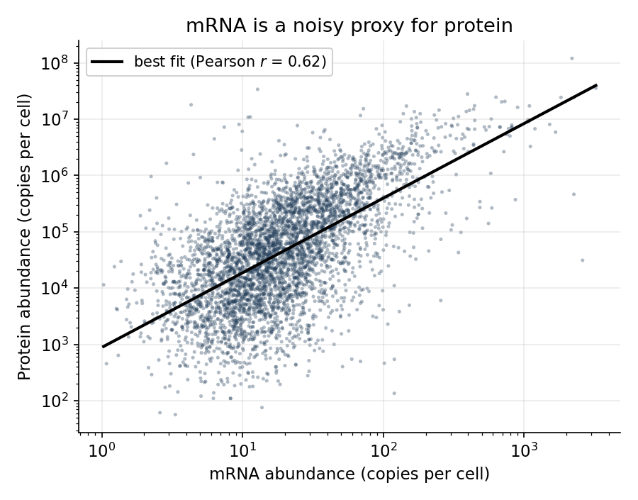
Figure 2: mRNA is a noisy proxy for protein. Real per-gene mRNA and protein copy numbers in mouse NIH3T3 fibroblasts (Schwanhäusser et al. 2011; \(n=4{,}309\) genes; Pearson \(r=0.62\) on log abundances). The red line is the best fit; even so, protein scatters across two to three orders of magnitude at any given mRNA level, because translation and degradation are not observed in the RNA.
Popular datasets
Below is a set of some of the most popular public datasets in genomics. File sizes can be quite large — for WGS, FASTQ files are often around 100-200GB, BAM files are 30-100GB, and VCF files are 1-10GB. However, as described earlier, much of this information represents redundancy with the reference genome, and individuals are often the unit of interest when training AI models rather than nucleotides, so cohort sizes in the thousands-hundreds of thousands range is often fairly small for modern AI. Additionally, most data are collected on healthy individuals or individuals with cancer, so it is difficult to study other diseases because public datasets will be quite small (if available at all). And any data collected from a single institution or region will have batch effects, limiting generalizability to other populations.
| Resource | What it is | Assay | Reported scale | Ref. |
|---|---|---|---|---|
| 1000 Genomes | Reference catalogue of human variation | WGS, WES | 2,504 individuals, 26 populations; ~88M variants | 1 |
| gnomAD | Aggregated exomes + genomes; constraint metrics | WES, WGS | 125,748 exomes + 15,708 genomes (v2) | 10 |
| UK Biobank | Population cohort, genotype + deep phenotype | Array, WES, WGS | ~500,000 participants | 11 |
| TCGA | Pan-cancer tumor/normal multi-omics | WXS, WGS, bulk RNA-seq, WSI | ~11,000 tumors, 33 cancer types | 12 |
| GTEx | Genetic regulation of expression across tissues | bulk RNA-seq, WGS | 17,382 RNA-seq samples, 54 tissues, 948 donors | 13 |
| ENCODE | Functional/regulatory element annotation | ChIP-seq, ATAC, DNase, RNA-seq | Genome-wide assays across many cell types | 14 |
| GENCODE | Reference gene/transcript annotation | Annotation | ~20,000 coding genes; >200,000 transcripts | 15 |
| Geuvadis | RNA-seq paired to 1000 Genomes genotypes | bulk RNA-seq | 462 individuals, 5 populations | 16 |
| Tabula Sapiens | Multi-organ single-cell atlas | scRNA-seq | ~500,000 cells, ~24 tissues | 17 |
| CZ CELLxGENE Discover | Aggregated, standardized single-cell expression atlas | scRNA-seq | >90M cells across thousands of datasets | 18 |
| Human Cell Atlas | Cross-tissue single-cell reference of every cell type | scRNA-seq | Tens of millions of cells across many tissues | 19 |
| 10x Genomics Datasets | Vendor-released public single-cell/-nucleus datasets | scRNA-seq | Hundreds of datasets across tissues | 20 |
| T2T-CHM13 | First complete (telomere-to-telomere) human genome | WGS (long-read) | 1 gapless assembly | 21 |
Assay abbreviations: WGS = whole-genome sequencing; WES/WXS = whole-exome sequencing; bulk RNA-seq = bulk RNA sequencing; scRNA-seq = single-cell RNA sequencing; Array = genotyping microarray; WSI = whole-slide imaging; ChIP-seq = chromatin immunoprecipitation sequencing; ATAC = assay for transposase-accessible chromatin; DNase = DNase I hypersensitivity sequencing.
Two structural problems run underneath these numbers.
How real models approach this
We’ve talked a lot about how genetic material can be represented as text for AI models. But what is actually done in practice? Here are a few notable examples.
- AlphaFold2 (Jumper et al.22) predicts protein three-dimensional (3D) structure from amino-acid sequence at near-experimental accuracy — arguably the field’s defining success. It takes a protein’s amino-acid sequence, together with a multiple-sequence alignment of evolutionarily related proteins and any available structural templates, and predicts the 3D coordinates of every atom. The sequence is treated as a string over the fixed 20-letter amino-acid alphabet — each residue is mapped to a learned embedding rather than an arbitrary text token — and much of the biological signal comes from the MSA, whose column-wise evolutionary covariation encodes which residues are likely to contact one another in 3D. Protein folding is a problem that possesses multiple attributes that make it an ideal candidate for AI. The 3D structure depends entirely on the discrete amino acid sequence itself, without dependencies from other parts of the genome or cell state broadly. There are over 200,000 experimentally determined protein structures with resolved amino-acid sequences across humans and model organisms23, representing a dataset that is large enough for supervised learning. And amino acids have biochemical properties that enable logical verification of predicted results to an extent.
- Enformer24 and AlphaGenome25 attack the cis-regulatory problem head-on, predicting expression and chromatin readouts from sequence across ~200 kilobases and up to 1 megabase windows respectively. They are the state of the art on long-range cis effects — and structurally blind to trans regulation that acts through diffusible proteins or other chromosomes. Both take a one-hot-encoded DNA sequence — a long genomic window centered on the region of interest — and predict thousands of functional genomic and epigenomic tracks (expression, chromatin accessibility, histone marks, and more) along that window. Here the alphabet is simply the four DNA bases (A/C/G/T): each position becomes a 4-dimensional one-hot vector, so — unlike a text model with a learned subword vocabulary — there is no tokenization step at all, and biology enters through the fixed base alphabet and the reverse-complement symmetry the architectures are built to respect (a sequence and its complementary strand should give the same prediction).
- DNABERT26, the Nucleotide Transformer27, and Evo28 are DNA “language models” — masked or autoregressive pre-training over genomic sequence, transferred to downstream tasks. Each tokenizes raw nucleotide sequence — overlapping k-mers for DNABERT, fixed non-overlapping k-mer tokens for the Nucleotide Transformer, and single-nucleotide (byte-level) tokens for Evo — and learns representations by predicting masked or next tokens over large genomic corpora. The vocabulary is built from the four nucleotides rather than natural-language words, and the differing tokenizations are attempts to package that four-letter alphabet into biologically meaningful units: k-mers approximate short motifs or codon-like chunks, while single-base tokens keep every nucleotide addressable at the cost of longer sequences.
- scGPT29 and Geneformer30 bring the foundation-model recipe to single-cell transcriptomics, learning representations of cell state from large RNA-expression atlases. These approaches do not take in raw sequencing reads as input, but rather the processed count matrices. Consequently the “alphabet” is not sequence at all but the roughly 20,000 genes — each gene is a token, and its expression level is encoded either by binning the count into discrete value tokens (scGPT) or by ranking genes from most to least expressed within a cell (Geneformer), so the biology is carried by which genes are on and their relative levels rather than by any letter sequence.
Conclusion
There have been exciting developments in genomics AI, and there is much to be done moving forward. ~40% of variants in cancer cases are still classified as variants of unknown significance31. When analyzing a cancer patient’s mutations, it is still often impossible to distinguish the driver mutation from passenger mutations. The role of genomics outside of cancer and well-characterized genes characterized by single mutation/gene events is minimal in clinical practice. A single human scRNA-seq experiment often has thousands of cells, and tens of thousands of genes. In an atlas comprised of dozens or hundreds of datasets, there can be millions of cells, with various sources of batch effects. Continuing to develop models that can make sense of these data will be critical for advancing genomics research.
References
-
The human reference genome disproportionately represents individuals of European ancestry, as these are the most widely available genomic data. Recent efforts have been made to create pan-genomes that better represent global diversity, most notably the Human Pangenome Reference Consortium’s draft reference assembled from 47 genetically diverse individuals2. ↩
Reproduce all analyses in this post here.
All writing is my own. AI was not used to write this post.
Leave a Comment