<?xml version="1.0" encoding="utf-8"?><feed xmlns="http://www.w3.org/2005/Atom" ><generator uri="https://jekyllrb.com/" version="4.4.1">Jekyll</generator><link href="https://joseph-rich.com/feed.xml" rel="self" type="application/atom+xml" /><link href="https://joseph-rich.com/" rel="alternate" type="text/html" /><updated>2026-06-02T01:01:28+00:00</updated><id>https://joseph-rich.com/feed.xml</id><title type="html">Joseph Rich</title><subtitle>Blog and writing by Joseph Rich on machine learning, bioinformatics, and radiology.</subtitle><author><name>Joseph Rich</name><email>josephrich98@gmail.com</email></author><entry><title type="html">Genomics Is Not NLP: A Field Guide for ML Scientists</title><link href="https://joseph-rich.com/posts/2026/06/genomics-vs-nlp/" rel="alternate" type="text/html" title="Genomics Is Not NLP: A Field Guide for ML Scientists" /><published>2026-06-03T00:00:00+00:00</published><updated>2026-06-03T00:00:00+00:00</updated><id>https://joseph-rich.com/posts/2026/06/genomics-vs-nlp</id><content type="html" xml:base="https://joseph-rich.com/posts/2026/06/genomics-vs-nlp/"><![CDATA[<!-- Generated from posts/genomics-vs-nlp/main.md by scripts/sync_posts.py. Do not edit here; edit the source and re-commit. -->

<h1 id="why-a-language-model-experts-intuitions-misfire">Why a language-model expert’s intuitions misfire</h1>

<p>DNA is the most beguiling analogy in all of machine learning. It is a string. It
is written in a tiny alphabet. You read it left to right. It has motifs that look
like words, genes that look like sentences, and a “grammar” that biologists have
spent a century annotating. If you have trained transformers on text, the leap to
genomics feels like a short one — same architecture, new corpus.</p>

<p>It is not a short one. The architectures really do carry over (transformers,
state-space models, masked-language-model pre-training, increasingly genomic
“foundation models”), which is exactly what makes the analogy dangerous: it hides
everything that is different. This post is a field guide for machine-learning
scientists moving from natural language into genomics and transcriptomics. What
changes is not the network. It is the statistics of the signal, the meaning of a
“token,” the fact that the entire species shares essentially one sequence, the
biology you must encode to read a single variant, and — the part that quietly
sinks most projects — <strong>the molecule you can cheaply measure is not the molecule
that actually does anything.</strong></p>

<p>A running theme, the mirror image of the one I used for radiology:
some things here are genuinely <em>easier</em> than language, and a few are
catastrophically harder. (For the imaging counterpart of this argument, see
<a href="/posts/2026/06/radiology-ai-vs-computer-vision/">Radiology AI Is Not Computer Vision</a>.)
Knowing which is which is the difference between a model that tops a benchmark and
one that says something true about biology.</p>

<h1 id="the-alphabet-is-tiny--and-stranger-than-text">The alphabet is tiny — and stranger than text</h1>

<p>Start with the surface, because the surface is where the false comfort lives.</p>

<p>Line up like with like before drawing the comparison. The right counterpart to
DNA’s <strong>four</strong> letters — \(\{A, C, G, T\}\), with RNA swapping \(T\) for \(U\) — is not
an NLP tokenizer’s 32,000–100,000-token vocabulary but the <strong>26 letters of
written English</strong>: both are the raw character set from which everything else is
assembled. On <em>that</em> axis DNA’s alphabet is merely small, not exotic. The
comparison only gets interesting one level up, at the <em>word</em> — and there the
genome’s closest analogue is the <strong>gene</strong>, of which humans have only ~20,000
(Section 7), each one hundreds to thousands of letters long rather than five. So a
four-letter alphabet “sounds like a gift,” and for sheer per-symbol modeling
capacity it is — but the comfort is misplaced, because the difficulty was never in
the alphabet. Three wrinkles make even the alphabet less clean than it looks.</p>

<p><strong>It is not really four symbols.</strong> Real sequence files are littered with <code class="language-plaintext highlighter-rouge">N</code>, the
“any base” placeholder for positions the sequencer could not call, and with the
full IUPAC ambiguity set (<code class="language-plaintext highlighter-rouge">R</code> = A or G, <code class="language-plaintext highlighter-rouge">Y</code> = C or T, <code class="language-plaintext highlighter-rouge">W</code>, <code class="language-plaintext highlighter-rouge">S</code>, <code class="language-plaintext highlighter-rouge">K</code>, <code class="language-plaintext highlighter-rouge">M</code>, and so
on) for positions known to be one of a subset. On top of that, reference genomes
use <strong>case to encode a second channel</strong>: lowercase <code class="language-plaintext highlighter-rouge">acgt</code> marks soft-masked
regions — repeats and low-complexity sequence flagged by tools like RepeatMasker —
while uppercase marks the rest. So <code class="language-plaintext highlighter-rouge">a</code> and <code class="language-plaintext highlighter-rouge">A</code> are the <em>same base</em> carrying
<em>different metadata</em>. A tokenizer that uppercases everything silently discards a
curated annotation; one that treats <code class="language-plaintext highlighter-rouge">a</code> and <code class="language-plaintext highlighter-rouge">A</code> as distinct tokens doubles the
alphabet for the wrong reason. Neither is obviously right, and the choice is yours
to make consciously.</p>

<p><strong>The hard axis is length, not alphabet.</strong> This inverts the usual NLP scaling
axis: there is almost nothing to learn about the <em>alphabet</em>; all the difficulty is
in the <strong>length</strong>. The haploid human genome is about
\(3.2 \times 10^{9}\) base pairs — a single “document” of 3.2 billion characters,
two to three orders of magnitude longer than the entire training context of a
long-context LLM. This is why tokenization is a live research question in genomics
in a way it is not for English: single-nucleotide tokens give you faithful
resolution but punishing sequence lengths; \(k\)-mer tokens (e.g. 6-mers) or
byte-pair encodings shorten the sequence but blur the single-base substitutions
that often <em>are</em> the signal. The thing you most want to detect — a one-letter
change — is the thing aggressive tokenization destroys.</p>

<p><strong>The string has a symmetry text does not.</strong> DNA is double-stranded, and the two
strands carry the same information in complementary, reverse-ordered form: the
reverse complement of <code class="language-plaintext highlighter-rouge">5'-GATTACA-3'</code> is <code class="language-plaintext highlighter-rouge">5'-TGTAATC-3'</code>. A gene can live on
either strand, so a motif and its reverse complement are often biologically
equivalent — an equivariance with no analogue in natural language, where reading a
sentence backwards through a letter-substitution cipher is gibberish. Good genomic
models build in reverse-complement equivariance (or augment with it); naive ones
waste capacity relearning each motif twice. Relatedly, <strong>strand bias</strong> — the two
strands accruing mutations or being sequenced at different rates — is a real
artifact you must model, not a nuisance you can normalize away.</p>

<h1 id="almost-every-genome-is-the-same-genome">Almost every genome is the same genome</h1>

<p>Here is the single biggest statistical difference from a text corpus, and it runs
exactly opposite to intuition. Two English documents pulled at random share almost
nothing at the token level. <strong>Two human genomes are 99.9% identical.</strong></p>

<p>
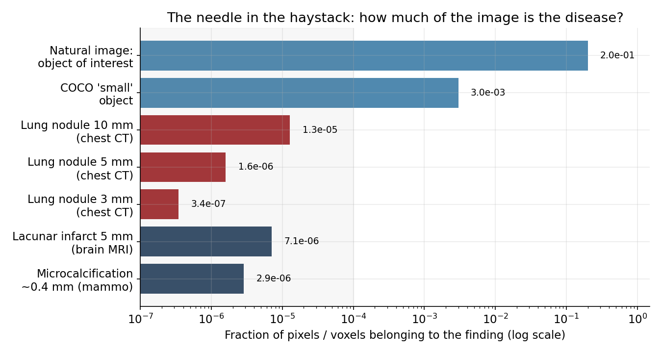
Pairwise nucleotide diversity in humans is about \(\pi \approx 0.001\): roughly one
site in a thousand differs between any two people. Across \(3.2 \times 10^{9}\)
bases, a typical genome carries on the order of <strong>4–5 million</strong> sites that differ
from the reference — which sounds like a lot until you remember it is \(0.1\%\) of
the sequence. The other \(99.9\%\) is, position for position, the same book. Figure 1a
puts this on a log axis against the divergence you would see between species
(\(\sim 1.2\%\) human–chimpanzee) and against text, where two unrelated documents
differ at essentially every token.
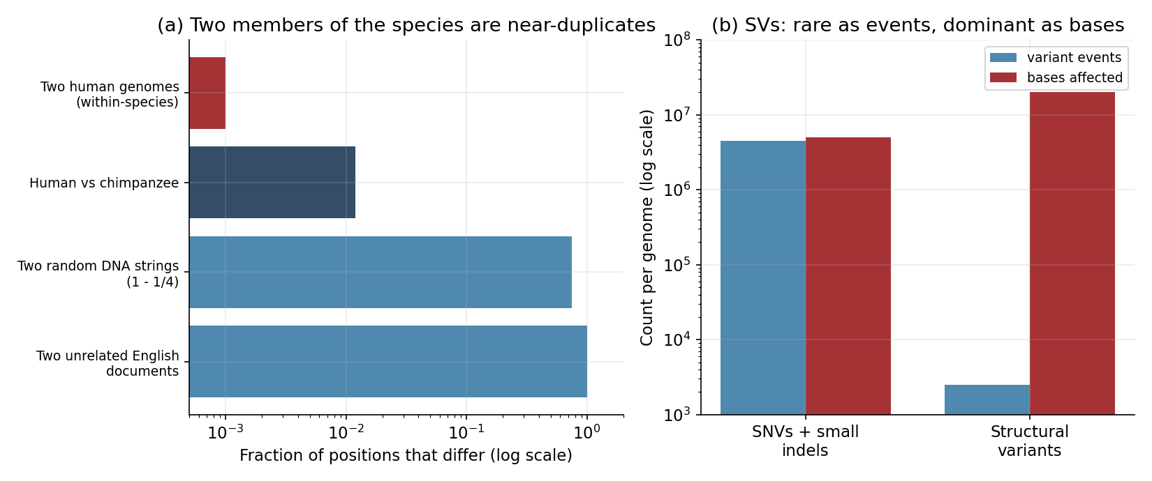
</p>

<p><img src="/images/posts/genomics-vs-nlp/corpus_redundancy.png" alt="**Figure 1.** The corpus is nearly one document. **(a)** The fraction of
positions that differ between two sequences, log scale: two humans differ at
$$\sim 10^{-3}$$, human and chimpanzee at $$\sim 10^{-2}$$, while two random DNA
strings differ at $$0.75$$ and two unrelated English documents at essentially $$1$$.
The within-species genomic &quot;corpus&quot; is roughly a thousandfold more redundant than
text. **(b)** Within one genome, single-nucleotide variants and small indels
dominate as *events* ($$\sim 4.5\text{M}$$) but touch only a few Mb; structural variants are
rare as events ($$\sim 2{,}500$$) yet rearrange $$\sim 20\,\mathrm{Mb}$$ — the majority of the bases
that actually differ, and the least
studied." /></p>

<p><strong>Why so uniform?</strong> Human genetic variation is shallow because the population that
gave rise to everyone alive passed through a long period of small <strong>effective
population size</strong> (\(N_e\) on the order of \(10^{4}\)) and a series of out-of-Africa
bottlenecks tens of thousands of years ago (conventionally placed
\(\sim 50{,}000\text{–}70{,}000\) years ago). The practical consequence for a modeler is
profound: <strong>the common variants you see are old and shared.</strong> They are ancestral
polymorphisms that predate the bottleneck, inherited by everyone and merely
<em>reshuffled</em> into new combinations by recombination each generation. There is not
a fresh, independent draw of variation per person; there is one ancestral deck,
dealt and re-dealt. On top of that shared deck, each newborn carries only
<strong>dozens</strong> of brand-new mutations — about 70 <em>de novo</em> single-nucleotide variants
per generation, from a per-base mutation rate near \(1.2 \times 10^{-8}\). So a
person is: the ancestral common variants (shuffled) \(+\) a small private set of
rare and <em>de novo</em> ones.</p>

<p>There is a second subtlety in <em>which</em> differences you are counting (Figure 1b).
Count variation by <strong>events</strong> and single-nucleotide variants (SNVs) and small
indels dominate — millions of them. Count it by <strong>bases affected</strong> and the picture
flips: a typical genome harbors only a couple of thousand <strong>structural variants</strong>
(deletions, duplications, inversions, insertions of mobile elements), but those
rearrange roughly <strong>20 Mb</strong> of sequence — far more nucleotide content than all the
SNVs combined. Structural variants are simultaneously the largest source of
differing bases and the <em>least</em> studied, because they are hard to call from short
reads and awkward to represent against a single linear reference. Much of the
“missing” signal in genomics lives in exactly the variation our tooling sees
worst.</p>

<p>For an ML scientist, the redundancy is not a curiosity — it is a <strong>data-leakage
hazard that dwarfs anything in NLP</strong>:</p>

<ul>
  <li><strong>Your training and test “documents” are near-identical by construction.</strong> A
random train/test split over individuals leaves the two sets sharing \(99.9\%\) of
their sequence and the overwhelming majority of their common variants. A model
can score brilliantly by memorizing ancestral haplotypes that appear on both
sides of the split.</li>
  <li><strong>Relatedness and population structure are confounders, not noise.</strong> Cryptic
relatives, or simply two people of shared ancestry, share long haplotype blocks.
This is the genomic analogue of a radiology model learning the scanner instead of
the disease: here the model learns <em>ancestry</em> and launders it as signal. Split by
family and, where the question demands it, by population; correct for structure
with principal components or mixed models; and never trust an evaluation that
could be won by recognizing where someone’s grandparents were born.</li>
  <li><strong>The reference itself is a bias.</strong> Mapping everyone to one linear reference
genome systematically mishandles the variants — especially structural ones —
that the reference happens not to contain. Pangenome graph references exist to
fight this; ignoring it bakes a population-specific blind spot into your inputs.</li>
</ul>

<h1 id="most-of-the-genome-is-unread--and-the-labels-need-a-wet-lab-or-a-patient">Most of the genome is unread — and the labels need a wet lab or a patient</h1>

<p>In a text corpus, every token means something to a competent human reader; meaning
is <em>in distribution</em> to the annotator. Genomics is not like this. Only about
\(1\)–\(2\%\) of the human genome codes for protein. The rest is introns, regulatory
elements, structural and repetitive sequence, and vast stretches whose function is
genuinely unknown. The ENCODE project assigned “biochemical activity” to most of
the genome, but biochemical activity is not the same as <em>function</em>, and the
fraction of the genome whose role we can actually read off remains small. Most of
the book is written in a language we have only begun to decode.</p>

<p>This reshapes what “supervised learning” can even mean, because the <strong>labels are
the bottleneck</strong>, just as annotation is in radiology — and for a deeper reason than
cost:</p>

<ul>
  <li><strong>Function is not in the sequence the way meaning is in the text.</strong> You cannot
look at a 200-base enhancer and read its effect the way you can read a sentence.
Establishing what a non-coding region <em>does</em> requires a wet-lab experiment — a
massively parallel reporter assay, a CRISPR perturbation screen, a knockout — or
a population-scale association to a phenotype. The label lives in an experiment or
in a patient, not in the characters.</li>
  <li><strong>“Ground truth” is often officially uncertain.</strong> Clinical variant databases
enshrine this honesty: a large share of catalogued variants are <strong>Variants of
Uncertain Significance (VUS)</strong> — we have seen them but cannot say whether they
cause disease. Pathogenicity calls follow formal guidelines (ACMG/AMP), yet
different labs reach <em>conflicting</em> classifications for the same variant often
enough that reconciling them is its own field. If your training labels are
pathogenic/benign calls, you are inheriting both the biology’s uncertainty and the
curators’ disagreement — the genomic version of inter-reader variability.</li>
  <li><strong>You cannot eyeball the data.</strong> An NLP engineer can sanity-check a labeling
pipeline by reading examples. Almost no one can look at a stretch of intron and
tell whether a splice-site annotation is right. As in radiology, you need a
biologist in the loop continuously, because the data-cleaning decisions
(which transcripts to keep, how to treat a multi-mapping read, what counts as
“expressed”) are biological judgments wearing a data-engineering disguise.</li>
</ul>

<h1 id="meaning-travels-cis-trans-and-the-limits-of-a-context-window">Meaning travels: cis, trans, and the limits of a context window</h1>

<p>The defining structural fact of language modeling over the last few years has been
the <strong>expanding context window</strong> — from a few thousand tokens to a million and
beyond — on the premise that if a dependency exists, a long enough window will span
it. Genomics tempts you to apply the same logic, and to a point it works: the
state-of-the-art regulatory models read enormous windows. Enformer takes about
\(200\,\mathrm{kb}\) of sequence; DeepMind’s 2025 <strong>AlphaGenome</strong> ingests up to
\(\sim 1\,\mathrm{Mb}\) — a literal one-million-base context window — to predict
regulatory activity. The parallel to long-context LLMs is exact, and deliberate.</p>

<p>But a linear window, however long, runs into a wall that has no NLP analogue,
because genomic regulation is <strong>not confined to a line</strong>:</p>

<ul>
  <li><strong>Cis-regulation is long-range but at least on-chromosome.</strong> Enhancers routinely
act over hundreds of kilobases, skipping past nearer genes to their true targets.
A \(1\,\mathrm{Mb}\) window is a real attempt to capture this — and it captures a
lot of it.</li>
  <li><strong>The genome is folded in 3D.</strong> Promoters and enhancers are brought into contact
by chromatin looping within topologically associating domains. Two elements far
apart on the sequence can be physically adjacent in the nucleus. Linear distance
in your input is not regulatory distance in the cell.</li>
  <li><strong>Trans-regulation breaks the line entirely.</strong> A transcription factor encoded on
chromosome 1 diffuses through the nucleus and binds targets on <em>every</em> chromosome.
<em>Trans</em>-eQTLs — variants that affect the expression of genes far away, often on
other chromosomes — are exactly this. No sliding window over a single locus, of
any length, can see a regulator that lives on a different chromosome and acts
through a <em>protein intermediate that is not in the input sequence at all</em>.</li>
</ul>

<p>That last clause is the crux. In language, the relevant context is always more
<em>text</em>; a bigger window is the right tool. In genomics, the relevant context is
frequently a <strong>diffusible molecule, a 3D contact, or a cell-state variable</strong> that
the DNA sequence does not contain. The state that determines what a sequence does
is not fully written in the sequence. Stretching the context window from
\(200\,\mathrm{kb}\) to \(1\,\mathrm{Mb}\) is genuine progress on the <em>cis</em> problem and
buys nothing on the <em>trans</em> problem. Be precise about which one your model is
actually solving.</p>

<h1 id="you-cannot-read-the-data-without-biology">You cannot read the data without biology</h1>

<p>This is the section a language modeler is most tempted to skip and least able to
afford skipping. A handful of biological facts are not background color; they
change what a model <em>must</em> represent to be correct.</p>

<p><strong>The reading frame and the genetic code.</strong> Protein-coding sequence is read in
non-overlapping triplets (<strong>codons</strong>). With four letters, there are \(4^3 = 64\)
codons mapping onto 20 amino acids plus stop — a <strong>degenerate</strong> code, so several
codons specify the same amino acid (most often differing in the third “wobble”
position). Three consequences follow immediately: the code is frame-dependent (an
insertion or deletion not divisible by three causes a <strong>frameshift</strong> that garbles
everything downstream); the same protein can be written many ways; and a model
operating on raw nucleotides has to <em>learn</em> a triplet structure that is given, not
discovered.</p>

<p><strong>Silent does not mean neutral.</strong> Because the code is degenerate, a single-base
change can be <strong>synonymous</strong> (“silent”) — it leaves the amino acid unchanged. The
naive inference is that synonymous variants do not matter. They often do: they can
alter codon-usage and translation efficiency, mRNA folding and stability, and —
crucially — they can create or destroy <strong>splice signals</strong>. The hierarchy a model
should encode is <em>synonymous / missense / nonsense</em>, but with the explicit caveat
that “synonymous” is a statement about the protein sequence, not about function.</p>

<p><strong>Splicing and RNA processing.</strong> The path from gene to message is not a copy. A
pre-mRNA is <strong>spliced</strong> — introns removed, exons joined — then capped at the
\(5'\) end and polyadenylated at the \(3'\). A variant deep inside an intron, far from
any coding base, can create a <strong>cryptic splice site</strong> and ruin a protein; a variant
at an exon boundary can cause <strong>exon skipping</strong>. This is why “distance to the
nearest coding base” is a terrible proxy for “importance,” and why models that
ignore splicing miss an entire mechanism of disease.</p>

<p><strong>Driver versus passenger.</strong> In cancer genomics the problem is explicitly a
signal-detection one. A tumor genome accumulates thousands of somatic mutations,
the vast majority of which are <strong>passengers</strong> — along for the ride, biologically
inert. A handful are <strong>drivers</strong> that actually confer growth advantage.
Distinguishing the few drivers from the many passengers, against a mutational
background that varies across the genome, is the central inference task — the
genomic needle-in-a-haystack.
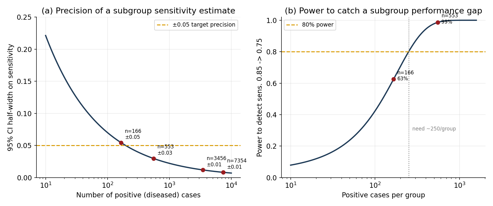
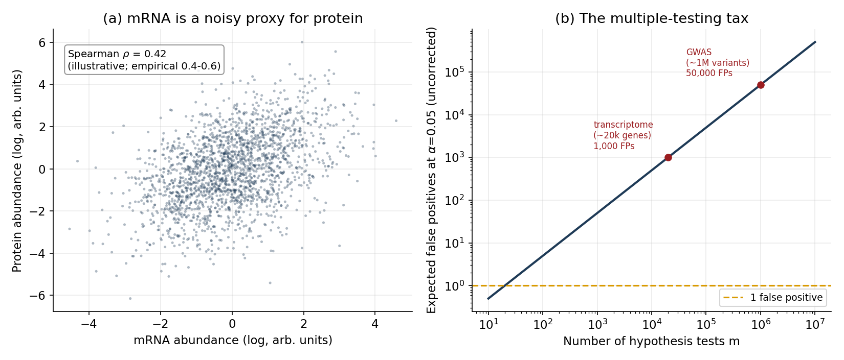
</p>

<p><strong>Multiple testing is not optional.</strong> When you test millions of variants for
association with a trait, or tens of thousands of genes for differential
expression, the number of hypotheses is so large that uncorrected \(p\)-values are
meaningless. This is why genome-wide association studies adopted a <strong>genome-wide
significance threshold of \(p &lt; 5 \times 10^{-8}\)</strong> — essentially a Bonferroni
correction for the \(\sim 10^{6}\) independent common-variant tests across the genome.
We return to the arithmetic in Figure 3b; for now, internalize that a “significant”
hit at \(p = 10^{-3}\) is, genome-wide, almost certainly noise.</p>

<p><strong>
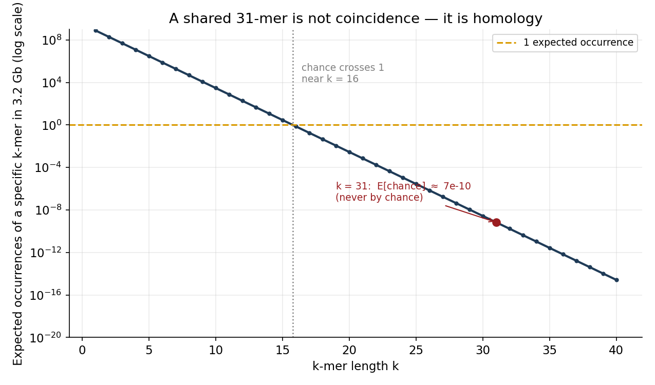
Sequence similarity runs far above chance — and that is the whole point.</strong> Here
is the calculation that should reframe how a string modeler thinks about DNA. Under
a naive model of i.i.d. uniform bases, a <em>specific</em> \(k\)-mer is expected to occur
\(G \cdot 4^{-k}\) times in a genome of \(G\) bases:</p>

\[\mathbb{E}[\text{occurrences}] = G \cdot 4^{-k}.\]

<p>For \(G = 3.2 \times 10^{9}\), this crosses \(1\) near \(k \approx 16\) and collapses fast
(Figure 2). At the \(k = 31\) that bioinformatics tooling routinely uses for exact
matching, the expected number of <em>chance</em> occurrences of a given 31-mer is</p>

\[3.2\times 10^{9} \cdot 4^{-31} \approx 7 \times 10^{-10},\]

<p>i.e. effectively never. And yet conserved 31-mers are shared <em>constantly</em> — between
two people, between human and mouse, across hundreds of millions of years of
divergence. The naive random-sequence model predicts these shared long \(k\)-mers
should not exist; they exist anyway, by a factor of a billion. <strong>That gap is
biology</strong>: purifying selection conserving functional sequence, preserved RNA
secondary structure constraining which substitutions are tolerated, conserved
amino-acid motifs (with synonymous wobble underneath), and repetitive elements
copied across the genome. The lesson is that string coincidence is the <em>wrong null</em>.
When two sequences match more than chance allows, that excess is the signal —
homology, conservation, selection — and a model that treats DNA as a random string
will systematically misread it.</p>

<p><img src="/images/posts/genomics-vs-nlp/kmer_chance.png" alt="**Figure 2.** Similarity beyond chance. Under an i.i.d.-uniform-base null, the
expected number of occurrences of a *specific* $$k$$-mer in a 3.2 Gb genome is
$$G\cdot 4^{-k}$$; it crosses $$1$$ near $$k \approx 16$$ and reaches
$$\approx 7\times 10^{-10}$$ at $$k = 31$$. Long $$k$$-mers therefore essentially never
recur by chance — so when they *are* shared between individuals or species, the
match is homology and conservation, not coincidence. The gap between this curve and
observed sequence sharing is exactly the biology a string model must
learn." /></p>

<h1 id="the-unit-problem-long-genes-many-transcripts-slippery-semantics">The unit problem: long genes, many transcripts, slippery semantics</h1>

<p>In language the semantic unit is convenient: a word is a few characters, a sentence
a few dozen words, and meaning is reasonably local and human-readable. The genomic
“word” is nothing like this.</p>

<p><strong>Genes are long, and their meaning is delocalized.</strong> A protein-coding sequence is
typically on the order of \(1\)–\(2\,\mathrm{kb}\) (encoding a protein of very roughly
\(\sim 375\) amino acids, with wide spread across the proteome), but the <em>gene</em> —
exons plus the introns between them — frequently spans tens to hundreds of
kilobases; dystrophin spans about \(2.2\,\mathrm{Mb}\). The information that
specifies one protein is scattered across a huge genomic interval, interrupted by
introns, and its realized “meaning” depends on cell type, developmental stage, and
regulatory state. Compared with a five-letter English word whose meaning is right
there on the page, the semantics of a gene are spread out, context-dependent, and
much harder to capture in a fixed embedding.</p>

<p><strong>One gene is many messages.</strong> It is common shorthand that humans have “about
20,000 genes” — and the protein-coding count, \(\sim 19{,}900\text{–}20{,}000\) in GENCODE, is
indeed remarkably small. But that number badly understates the functional
vocabulary, because <strong>alternative splicing</strong> lets a single gene produce many
distinct <strong>transcripts</strong> (isoforms). GENCODE annotates well over \(200{,}000\)
transcripts — an order of magnitude more than genes — and a single gene can yield
dozens of isoforms with different, sometimes opposing, functions. So the mapping
from “gene” to “thing that acts” is one-to-many, and a transcriptomic model that
collapses expression to the gene level is averaging over functionally distinct
products. The right unit is frequently the transcript, not the gene — and
transcript-level labels are scarcer and noisier.</p>

<h1 id="the-molecule-you-sequence-is-not-the-molecule-that-acts">The molecule you sequence is not the molecule that acts</h1>

<p>Now the deepest mismatch, and the one most likely to invalidate a confident
conclusion. <strong>Proteins do the work of the cell</strong> — they catalyze, signal,
transport, and build. DNA is the blueprint and RNA the working copy, but the actors
are proteins. And yet the overwhelming majority of “expression” data, and nearly
all of the trendy single-cell atlases, measure <strong>RNA</strong>, not protein. We routinely
study the script and infer the performance.</p>

<p>That inference is shakier than the field’s habits suggest. Across many careful
studies, the correlation between a gene’s mRNA level and its protein level is
<strong>moderate at best — typically a Spearman \(\rho\) in the \(0.4\)–\(0.6\) range</strong>, and
lower still when you look at changes over time rather than steady-state across
genes. Schwanhäusser and colleagues found mRNA explained well under half the
variance in protein abundance; Vogel and Marcotte, Liu, Beyer and Aebersold, and
Buccitelli and Selbach all converge on the same message — translation rates, protein
half-lives, and post-translational regulation drive a large share of protein levels
that mRNA simply does not see. Edfors and colleagues showed the relationship is
<em>gene-specific</em>: each gene has roughly its own mRNA-to-protein conversion factor, so
a single global model is wrong per gene. Figure 3a illustrates the consequence —
even at the optimistic end of that range, knowing a gene’s mRNA leaves its protein
level uncertain across a wide band.</p>

<p><img src="/images/posts/genomics-vs-nlp/proxy_and_testing.png" alt="**Figure 3.** Two reasons to be careful. **(a)** An illustrative mRNA-versus-
protein scatter at a Spearman correlation in the empirically reported range; even
here, fixing the mRNA level leaves protein spanning a wide band, because
translation and degradation are not observed in the RNA. **(b)** The multiple-
testing tax: expected false positives at $$\alpha = 0.05$$ *without* correction grow
linearly with the number of tests — about $$1{,}000$$ across a $$\sim 20\text{k}$$-gene
transcriptome and $$\sim 50{,}000$$ across a $$\sim 1\text{M}$$-variant GWAS — which is why
genome-wide significance is set near $$5\times 10^{-8}$$." /></p>

<p>So why does the field overwhelmingly sequence RNA if protein is what matters? Not
because anyone thinks RNA is the better readout — because of <strong>technology</strong>:</p>

<ul>
  <li><strong>RNA can be amplified; protein cannot.</strong> Reverse transcription plus PCR turns a
handful of molecules into a sequenceable library, so RNA-seq reaches single-cell
and even single-molecule sensitivity. There is no PCR for proteins — no way to
exponentially copy a polypeptide — so mass-spectrometry proteomics works with
whatever is in the sample.</li>
  <li><strong>RNA is genome-templated, so we know what to look for.</strong> Every transcript maps
back to a sequence we can align against a reference. Proteins must be inferred from
fragmentary peptide spectra, and the proteome’s enormous dynamic range means
abundant proteins drown out the rare ones we often care about most.</li>
  <li><strong>Throughput and cost.</strong> RNA-seq is cheap, standardized, and scales to millions of
cells; comprehensive single-cell proteomics is still hard, lower-throughput, and
far less complete.</li>
</ul>

<p>The honest framing is the same one that recurs throughout this post: we optimize a
convenient <strong>proxy</strong>. RNA abundance is to protein activity what a radiology label
mined from a report is to the underlying pathology — useful, scalable, and
systematically wrong in ways you must keep in view. A transcriptomic model that
reports “expression” is making a claim about the script; whether the performance
followed is a separate, and weaker, inference.</p>

<h1 id="the-data-a-near-duplicate-corpus-batch-effects-and-who-is-in-it">The data: a near-duplicate corpus, batch effects, and who is in it</h1>

<p>
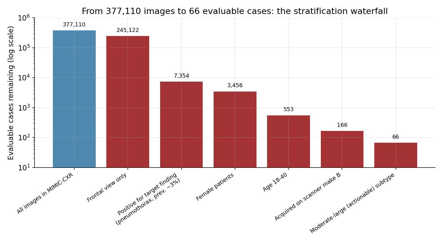
Genomics is, paradoxically, both data-rich and data-poor. There is an enormous and
growing public infrastructure (Table 1), far better than radiology’s. But the
redundancy of Section 3, the batch effects below, and the demographics of who has
been sequenced mean that <em>effective</em> sample size lags raw counts badly.</p>

<p>Table: Major public genomics / transcriptomics resources. Counts are as reported by
the source publications; “variants” and “samples” are not comparable units across
rows.</p>

<table>
  <thead>
    <tr>
      <th>Resource</th>
      <th>What it is</th>
      <th>Reported scale</th>
      <th>Citation (DOI)</th>
    </tr>
  </thead>
  <tbody>
    <tr>
      <td><strong>1000 Genomes</strong></td>
      <td>Reference catalogue of human variation</td>
      <td>2,504 individuals, 26 populations; ~88M variants</td>
      <td>10.1038/nature15393</td>
    </tr>
    <tr>
      <td><strong>gnomAD</strong></td>
      <td>Aggregated exomes + genomes; constraint metrics</td>
      <td>125,748 exomes + 15,708 genomes (v2)</td>
      <td>10.1038/s41586-020-2308-7</td>
    </tr>
    <tr>
      <td><strong>UK Biobank</strong></td>
      <td>Population cohort, genotype + deep phenotype</td>
      <td>~500,000 participants</td>
      <td>10.1038/s41586-018-0579-z</td>
    </tr>
    <tr>
      <td><strong>TCGA</strong></td>
      <td>Pan-cancer tumor/normal multi-omics</td>
      <td>~11,000 tumors, 33 cancer types</td>
      <td>10.1038/ng.2764</td>
    </tr>
    <tr>
      <td><strong>GTEx</strong></td>
      <td>Genetic regulation of expression across tissues</td>
      <td>17,382 RNA-seq samples, 54 tissues, 948 donors</td>
      <td>10.1126/science.aaz1776</td>
    </tr>
    <tr>
      <td><strong>ENCODE</strong></td>
      <td>Functional/regulatory element annotation</td>
      <td>Genome-wide assays across many cell types</td>
      <td>10.1038/nature11247</td>
    </tr>
    <tr>
      <td><strong>GENCODE</strong></td>
      <td>Reference gene/transcript annotation</td>
      <td>~20,000 coding genes; &gt;200,000 transcripts</td>
      <td>10.1093/nar/gkaa1087</td>
    </tr>
    <tr>
      <td><strong>Geuvadis</strong></td>
      <td>RNA-seq paired to 1000 Genomes genotypes</td>
      <td>462 individuals, 5 populations</td>
      <td>10.1038/nature12531</td>
    </tr>
    <tr>
      <td><strong>Tabula Sapiens</strong></td>
      <td>Multi-organ single-cell atlas</td>
      <td>~500,000 cells, ~24 tissues</td>
      <td>10.1126/science.abl4896</td>
    </tr>
    <tr>
      <td><strong>T2T-CHM13</strong></td>
      <td>First complete (telomere-to-telomere) human genome</td>
      <td>1 gapless assembly</td>
      <td>10.1126/science.abj6987</td>
    </tr>
  </tbody>
</table>

<p>Two structural problems run underneath these numbers.</p>

<p><strong>Batch effects are the scanner-heterogeneity of genomics.</strong> A sequencing readout
is the end of a long wet-and-dry pipeline, and every stage is a covariate that
shifts across labs: library preparation chemistry, sequencing platform (short-read
Illumina vs. long-read PacBio/Nanopore), read length and depth, PCR amplification
bias, RNA quality (RIN) and degradation, the alignment software, and — easy to
forget — the <strong>reference build</strong> itself (GRCh37 vs. GRCh38 vs. the new T2T-CHM13).
Two expression datasets can differ more by batch than by biology, and models
readily learn the batch. The discipline that grew up around this — careful
normalization, batch-correction methods, mixed models, harmonized pipelines — is
the genomic counterpart to vendor-aware augmentation and intensity normalization in
imaging. As there, the danger is symmetric: under-correct and you measure the lab;
over-correct and you erase the biology.</p>

<p><strong>The corpus is not representative of humanity.</strong> A large majority of participants
in genome-wide studies are of European ancestry. This is the genomic version of the
subgroup-power trap: a polygenic risk score trained predominantly on European-
ancestry data <strong>transfers poorly</strong> to people of other ancestries, because the tag
variants, allele frequencies, and linkage structure differ. A model can post
excellent aggregate metrics and still be least accurate for the populations most
underserved by existing tools. Splitting and evaluating <em>by ancestry</em>, and stating
plainly which groups you are and are not powered to serve, is not optional
diligence — it is the difference between a fair tool and an inequitable one.</p>

<h1 id="the-famous-models--and-what-they-do-and-dont-solve">The famous models — and what they do and don’t solve</h1>

<p>The reason this analogy is everywhere right now is that the transformer toolkit has
produced genuinely landmark genomics results. It is worth knowing the map, and being
precise about what each model does and does not address from the list above.</p>

<ul>
  <li><strong>AlphaFold2</strong> (Jumper et al., 2021) predicts protein 3D structure from amino-acid
sequence at near-experimental accuracy — arguably the field’s defining success. Note
what it sidesteps: it operates on the <em>protein</em>, taking the molecule that acts as a
given, and says nothing about whether or how much of that protein the cell makes.</li>
  <li><strong>Enformer</strong> (Avsec et al., 2021) and <strong>AlphaGenome</strong> (DeepMind, 2025) attack the
<em>cis</em>-regulatory problem head-on, predicting expression and chromatin readouts from
sequence across \(\sim 200\,\mathrm{kb}\) and up to \(\sim 1\,\mathrm{Mb}\) windows
respectively. They are the state of the art on long-range <em>cis</em> effects — and, per
Section 5, structurally blind to <em>trans</em> regulation that acts through diffusible
proteins or other chromosomes.</li>
  <li><strong>DNABERT</strong> (Ji et al., 2021), the <strong>Nucleotide Transformer</strong> (Dalla-Torre et al.,
2024), and <strong>Evo</strong> (Nguyen et al., 2024) are DNA “language models” — masked or
autoregressive pre-training over genomic sequence, transferred to downstream tasks.
They inherit, and must confront, every tokenization and redundancy issue in
Sections 2–3.</li>
  <li><strong>scGPT</strong> (Cui et al., 2024) and <strong>Geneformer</strong> (Theodoris et al., 2023) bring the
foundation-model recipe to single-cell <em>transcriptomics</em>, learning representations of
cell state from large RNA-expression atlases — which means they live entirely on the
RNA side of the proxy gap in Section 8.</li>
</ul>

<p>The pattern across the map is the through-line of this post: these models are
spectacular within the slice of the problem they address, and it is on the modeler to
know which slice that is. AlphaFold takes the protein as input; the regulatory models
see only <em>cis</em>; the single-cell models see only RNA. None of that diminishes them —
it just means the honest question is never “does the benchmark go up,” but “which part
of the biology did this actually capture, and which part is still missing.”</p>

<h1 id="takeaways">Takeaways</h1>

<p>If you remember five things moving from natural language to genomics:</p>

<ol>
  <li><strong>The alphabet is a trap, not a gift.</strong> Four letters (plus <code class="language-plaintext highlighter-rouge">N</code>, IUPAC codes, and
case-as-metadata), but the difficulty is the 3.2-billion-character length, the
reverse-complement symmetry, and a tokenization choice that can destroy the
single-base signal you came for.</li>
  <li><strong>The whole species is one near-duplicate corpus.</strong> Two genomes differ at \(0.1\%\)
of sites; common variants are old and shared, private variation is dozens of
mutations, and most differing <em>bases</em> hide in understudied structural variants.
Plan your splits around leakage, relatedness, and population structure from day one.</li>
  <li><strong>Most of the genome is unread, and labels live in experiments or patients.</strong>
Function is not in the sequence the way meaning is in text; ground truth is often an
official “uncertain,” and you cannot eyeball it. Keep a biologist in the loop.</li>
  <li><strong>Regulation defeats the context window.</strong> A \(1\,\mathrm{Mb}\) window is real
progress on <em>cis</em> and no progress on <em>trans</em>: the determining context is often a
protein, a 3D contact, or a cell state that the sequence does not contain.</li>
  <li><strong>You are usually modeling a proxy.</strong> RNA is not protein, and the correlation is
only \(\sim 0.4\)–\(0.6\); “expression” is the script, not the performance. Encode the
biology — codons, splicing, silent-but-not-neutral, drivers vs. passengers,
multiple testing, similarity-beyond-chance — or your string model will confidently
misread the genome.</li>
</ol>

<p>See the accompanying <code class="language-plaintext highlighter-rouge">notebook.ipynb</code> for the redundancy arithmetic, the \(k\)-mer
calculation, the proxy simulation, the multiple-testing counts behind Figures 1–3,
and an automated check that every citation below resolves.</p>

<h1 id="references">References</h1>

<ol>
  <li>Auton A, Brooks LD, Durbin RM, et al. A global reference for human genetic
variation. <em>Nature</em>. 2015;526(7571):68–74. doi:10.1038/nature15393</li>
  <li>Sudmant PH, Rausch T, Gardner EJ, et al. An integrated map of structural
variation in 2,504 human genomes. <em>Nature</em>. 2015;526(7571):75–81.
doi:10.1038/nature15394</li>
  <li>Karczewski KJ, Francioli LC, Tiao G, et al. The mutational constraint spectrum
quantified from variation in 141,456 humans. <em>Nature</em>. 2020;581(7809):434–443.
doi:10.1038/s41586-020-2308-7</li>
  <li>Bycroft C, Freeman C, Petkova D, et al. The UK Biobank resource with deep
phenotyping and genomic data. <em>Nature</em>. 2018;562(7726):203–209.
doi:10.1038/s41586-018-0579-z</li>
  <li>Weinstein JN, Collisson EA, Mills GB, et al. The Cancer Genome Atlas Pan-Cancer
analysis project. <em>Nat Genet</em>. 2013;45(10):1113–1120. doi:10.1038/ng.2764</li>
  <li>GTEx Consortium. The GTEx Consortium atlas of genetic regulatory effects across
human tissues. <em>Science</em>. 2020;369(6509):1318–1330. doi:10.1126/science.aaz1776</li>
  <li>ENCODE Project Consortium. An integrated encyclopedia of DNA elements in the
human genome. <em>Nature</em>. 2012;489(7414):57–74. doi:10.1038/nature11247</li>
  <li>Frankish A, Diekhans M, Jungreis I, et al. GENCODE 2021. <em>Nucleic Acids Res</em>.
2021;49(D1):D916–D923. doi:10.1093/nar/gkaa1087</li>
  <li>Lappalainen T, Sammeth M, Friedländer MR, et al. Transcriptome and genome
sequencing uncovers functional variation in humans. <em>Nature</em>.
2013;501(7468):506–511. doi:10.1038/nature12531</li>
  <li>Tabula Sapiens Consortium. The Tabula Sapiens: a multiple-organ, single-cell
transcriptomic atlas of humans. <em>Science</em>. 2022;376(6594):eabl4896.
doi:10.1126/science.abl4896</li>
  <li>Nurk S, Koren S, Rhie A, et al. The complete sequence of a human genome.
<em>Science</em>. 2022;376(6588):44–53. doi:10.1126/science.abj6987</li>
  <li>Kong A, Frigge ML, Masson G, et al. Rate of de novo mutations and the
importance of father’s age to disease risk. <em>Nature</em>. 2012;488(7412):471–475.
doi:10.1038/nature11396</li>
  <li>Schwanhäusser B, Busse D, Li N, et al. Global quantification of mammalian gene
expression control. <em>Nature</em>. 2011;473(7347):337–342. doi:10.1038/nature10098</li>
  <li>Vogel C, Marcotte EM. Insights into the regulation of protein abundance from
proteomic and transcriptomic analyses. <em>Nat Rev Genet</em>. 2012;13(4):227–232.
doi:10.1038/nrg3185</li>
  <li>Liu Y, Beyer A, Aebersold R. On the dependency of cellular protein levels on
mRNA abundance. <em>Cell</em>. 2016;165(3):535–550. doi:10.1016/j.cell.2016.03.014</li>
  <li>Edfors F, Danielsson F, Hallström BM, et al. Gene-specific correlation of RNA
and protein levels in human cells and tissues. <em>Mol Syst Biol</em>. 2016;12(10):883.
doi:10.15252/msb.20167144</li>
  <li>Buccitelli C, Selbach M. mRNAs, proteins and the emerging principles of gene
expression control. <em>Nat Rev Genet</em>. 2020;21(10):630–644.
doi:10.1038/s41576-020-0258-4</li>
  <li>Jumper J, Evans R, Pritzel A, et al. Highly accurate protein structure
prediction with AlphaFold. <em>Nature</em>. 2021;596(7873):583–589.
doi:10.1038/s41586-021-03819-2</li>
  <li>Avsec Ž, Agarwal V, Visentin D, et al. Effective gene expression prediction
from sequence by integrating long-range interactions. <em>Nat Methods</em>.
2021;18(10):1196–1203. doi:10.1038/s41592-021-01252-x</li>
  <li>Avsec Ž, Latysheva N, Cheng J, et al. AlphaGenome: advancing regulatory variant
effect prediction with a unified DNA sequence model. <em>bioRxiv</em>. 2025.
doi:10.1101/2025.06.25.661532. See also
https://deepmind.google/blog/alphagenome-ai-for-better-understanding-the-genome/</li>
  <li>Ji Y, Zhou Z, Liu H, Davuluri RV. DNABERT: pre-trained Bidirectional Encoder
Representations from Transformers model for DNA-language in genome.
<em>Bioinformatics</em>. 2021;37(15):2112–2120. doi:10.1093/bioinformatics/btab083</li>
  <li>Dalla-Torre H, Gonzalez L, Mendoza-Revilla J, et al. Nucleotide Transformer:
building and evaluating robust foundation models for human genomics. <em>Nat
Methods</em>. 2024;22(2):287–297. doi:10.1038/s41592-024-02523-z</li>
  <li>Nguyen E, Poli M, Durrant MG, et al. Sequence modeling and design from
molecular to genome scale with Evo. <em>Science</em>. 2024;386(6723):eado9336.
doi:10.1126/science.ado9336</li>
  <li>Cui H, Wang C, Maan H, et al. scGPT: toward building a foundation model for
single-cell multi-omics using generative AI. <em>Nat Methods</em>.
2024;21(8):1470–1480. doi:10.1038/s41592-024-02201-0</li>
  <li>Theodoris CV, Xiao L, Chopra A, et al. Transfer learning enables predictions in
network biology. <em>Nature</em>. 2023;618(7965):616–624.
doi:10.1038/s41586-023-06139-9</li>
</ol>

<hr />

<p><em>Reproduce all analyses in this post <a href="https://github.com/josephrich98/joseph_rich_blog/tree/main/posts/genomics-vs-nlp">here</a>.</em></p>]]></content><author><name>Joseph Rich</name><email>josephrich98@gmail.com</email></author><category term="machine learning" /><category term="genomics" /><category term="transcriptomics" /><category term="natural language processing" /><category term="computational biology" /><summary type="html"><![CDATA[A field guide for ML scientists moving into genomics and transcriptomics: why DNA only looks like text, why the whole species is one near-duplicate corpus, how regulation defeats the context window, the biology you cannot skip, why the molecule you sequence is not the one that acts, and what the famous foundation models do and don't solve.]]></summary></entry><entry><title type="html">Radiology AI Is Not Computer Vision: A Field Guide for ML Scientists</title><link href="https://joseph-rich.com/posts/2026/06/radiology-ai-vs-computer-vision/" rel="alternate" type="text/html" title="Radiology AI Is Not Computer Vision: A Field Guide for ML Scientists" /><published>2026-06-02T00:00:00+00:00</published><updated>2026-06-02T00:00:00+00:00</updated><id>https://joseph-rich.com/posts/2026/06/radiology-ai-vs-computer-vision</id><content type="html" xml:base="https://joseph-rich.com/posts/2026/06/radiology-ai-vs-computer-vision/"><![CDATA[<!-- Generated from posts/radiology-ai-vs-computer-vision/main.md by scripts/sync_posts.py. Do not edit here; edit the source and re-commit. -->

<h1 id="why-a-computer-vision-experts-intuitions-misfire">Why a computer-vision expert’s intuitions misfire</h1>

<p>If you have trained a model on ImageNet, COCO, or a few hundred million
Instagram photos, you have excellent instincts for natural-image vision. Most of
those instincts are wrong — or at least dangerously incomplete — the moment you
point them at a chest CT or a screening mammogram.</p>

<p>This post is a field guide for machine-learning scientists moving into
radiology. It is not a survey of architectures; the architectures are mostly the
ones you already know (CNNs, U-Nets, vision transformers, increasingly
foundation models). What changes is everything <em>around</em> the architecture: the
statistics of the signal, the cost and meaning of a label, the data you can
actually get, and — the part that quietly sinks most projects —
<strong>generalization across the bewildering heterogeneity of how medical images are
produced.</strong> I will end with the two things ML scientists most often discover too
late: how the FDA actually regulates these models, and why the model in the
paper is rarely the model that ships.</p>

<p>A running theme: medical imaging is in some ways <em>easier</em> than natural-image
vision, and leaning on those advantages is the difference between a model that
demos well and one that survives contact with a second hospital.</p>

<h1 id="what-is-genuinely-easier-than-natural-images">What is genuinely easier than natural images</h1>

<p>Start with the good news, because it is real and underexploited.</p>

<p><strong>Canonical pose and framing.</strong> A street scene can contain a cat at any scale,
any orientation, anywhere in the frame, against any background. A PA chest
radiograph is, by protocol, a patient standing upright, facing the detector,
arms positioned to rotate the scapulae off the lung fields. The heart is on the
left.<sup id="fnref:situs"><a href="#fn:situs" class="footnote" rel="footnote" role="doc-noteref">1</a></sup> The aortic knob is where the aortic knob goes. This is a strong
spatial prior that natural-image models simply do not get for free — and it is
why registration, atlas-based priors, and even fixed positional encodings work
far better here than they would on web images.</p>

<p><strong>One channel, calibrated.</strong> Most modalities are grayscale, and — crucially —
the gray values often <em>mean something physical</em>. CT is quantitative: each voxel
is a Hounsfield unit, a linear transform of the X-ray attenuation coefficient
\(\mu\) relative to water,</p>

\[\mathrm{HU} = 1000 \times \frac{\mu - \mu_{\text{water}}}{\mu_{\text{water}} - \mu_{\text{air}}},\]

<p>so water is \(0\), air is \(-1000\), fat is around \(-100\), and cortical bone is
\(+1000\) or more. Fat is fat in every CT scanner on Earth. Nothing in RGB is
calibrated like this; “how blue is the sky” is not a physical constant. You can
and should exploit it — windowing, HU-based preprocessing, and physically
motivated augmentations all follow from it.</p>

<p><strong>The suspected disease localizes attention.</strong> Clinical imaging arrives with a
<em>reason for exam</em>. “Rule out pneumothorax” tells you to look at the pleural line;
“rule out stroke” sends you to the brain parenchyma and vessels. The organ of
interest is usually known, which is a luxury object detection never has.</p>

<p>But each of these advantages has a barb:</p>

<ul>
  <li>The canonical pose breaks for portable/supine films, pediatric patients, body
habitus, and post-surgical anatomy.</li>
  <li>HU calibration drifts with scanner, kVp, and contrast timing (more on this
below), and MRI intensities are <em>not</em> standardized at all — a T1 value is only
meaningful relative to the rest of that one acquisition.</li>
  <li>“The organ of interest is known” is a trap: incidental findings in the
<em>other</em> organs are often what matter most clinically. The lung-nodule model
that ignores the adrenal mass at the edge of the field has failed the patient
even if its AUC is perfect.</li>
</ul>

<p>So: use the priors, but treat every one of them as a covariate that can shift.</p>

<h1 id="the-needle-in-the-haystack-subtlety-and-extreme-imbalance">The needle in the haystack: subtlety and extreme imbalance</h1>

<p>Here is the single biggest statistical difference from natural images. In
COCO, the object you care about typically occupies a meaningful fraction of the
frame. In radiology, the finding is often a handful of voxels in a sea of normal
tissue, and the difference between <em>malignant</em> and <em>benign</em> — between <em>call the
patient back</em> and <em>see you in two years</em> — can come down to a few millimeters of
spiculation or a subtle change in density.</p>

<p>Make it concrete with geometry. A chest CT of roughly \(512 \times 512 \times 320\)
voxels at \(0.7 \times 0.7 \times 1.0\,\text{mm}\) contains about \(8.4 \times 10^7\)
voxels. A clinically important \(5\,\text{mm}\) pulmonary nodule is a sphere of
volume \(\tfrac{4}{3}\pi r^3 \approx 65\,\text{mm}^3\), or about \(134\) voxels. The
lesion is therefore</p>

\[\frac{134}{8.4\times 10^7} \approx 1.6 \times 10^{-6}\]

<p>of the volume — roughly <strong>one in six hundred thousand voxels</strong>. Shrink it to a
\(3\,\text{mm}\) nodule and you are at one in <em>three million</em>. Figure 1 puts
several findings on the same axis as natural-image objects; note the five-to-six
order-of-magnitude gap.</p>

<p><img src="/images/posts/radiology-ai-vs-computer-vision/needle_in_haystack.png" alt="**Figure 1.** The fraction of an image that actually belongs to the finding,
on a log scale. Natural-image objects (blue) occupy $$10^{-3}$$ to $$10^{0}$$ of the
frame. Clinically critical lesions (red/navy) sit at $$10^{-7}$$ to $$10^{-5}$$.
This five-to-six order-of-magnitude difference is why naive pixel-wise losses
and patch samplers fail in radiology." /></p>

<p>The consequences for an ML scientist are direct:</p>

<ul>
  <li><strong>Accuracy is meaningless and pixel-wise loss is treacherous.</strong> A segmentation
model that predicts “no lesion” everywhere achieves \(1 - 1.6\times10^{-6}
\approx 99.9998\%\) voxel accuracy. Use overlap and detection metrics built for
imbalance — Dice / \(F_1\), where for prediction \(P\) and ground truth \(G\),
\(\mathrm{Dice} = \frac{2|P \cap G|}{|P| + |G|},\)
free-response ROC (FROC) for detection, and class-balanced or region-based
losses (Dice loss, Tversky, focal). The focal loss down-weights the easy
negatives that otherwise dominate the gradient:
\(\mathrm{FL}(p_t) = -(1-p_t)^{\gamma}\log p_t\).</li>
  <li><strong>Most of the volume is uninteresting, and uninteresting in a structured
way.</strong> Hard-negative mining, lesion-aware patch sampling, and two-stage
candidate-then-classify pipelines exist because uniformly sampling voxels
wastes almost all of your compute on obvious lung parenchyma.</li>
  <li><strong>Resolution is not negotiable.</strong> Downsampling a natural image to \(224^2\)
loses a cat’s whiskers; downsampling a CT slice can erase the lesion entirely.
The signal you are hunting may be at the Nyquist limit of the acquisition.</li>
</ul>

<h1 id="annotation-is-the-bottleneck-not-the-model">Annotation is the bottleneck, not the model</h1>

<p>In natural-image land, labels are cheap: crowdworkers draw boxes, and “is this a
dog” needs no credential. Radiology inverts this completely, and it reshapes
what is feasible.</p>

<p><strong>A bounding box is the wrong primitive, and often impossible.</strong> Many findings
have no crisp boundary. Where exactly does a ground-glass opacity end and normal
lung begin? What is the bounding box of diffuse interstitial disease, or of
“the lungs look hyperinflated”? The pathology is frequently a texture or a
<em>global</em> property, not a localizable object. Even when a lesion is discrete, it
lives in 3D — a box becomes a volume, and a radiologist scrolling 320 slices to
contour a tumour is spending clinical time that costs orders of magnitude more
than a crowdworker.</p>

<p><strong>Ground truth is noisy and sometimes unobtainable from the image alone.</strong> The
honest label often is not in the pixels. Is that lung nodule malignant? The
image cannot say; you need the biopsy, or two years of follow-up showing growth.
This is why so many “labels” in public datasets are actually <em>NLP-extracted from
the radiology report</em> (MIMIC-CXR, CheXpert, ChestX-ray14, PadChest all do this)
— which means your labels inherit both the radiologist’s error rate <em>and</em> the
text-mining model’s error rate.</p>

<p><strong>Inter-reader variability is a hard ceiling.</strong> Radiologists disagree. The
LIDC-IDRI lung-nodule database was annotated by four thoracic radiologists
precisely because no single read is ground truth; of 2,669 lesions marked as
nodules \(\geq 3\,\text{mm}\) by at least one reader, only about 35% were marked
by all four. If your “ground truth” is one radiologist, your evaluation noise
floor may be larger than the improvement you are claiming. Model the labels as
noisy: capture annotator agreement (e.g. Cohen’s / Fleiss’ \(\kappa\)), train
against multi-reader consensus where you can, and report performance relative to
the inter-reader band, not to an imagined perfect oracle.</p>

<p><strong>You cannot read the data without domain knowledge.</strong> A computer-vision
engineer can sanity-check an ImageNet pipeline by eye. Almost no ML scientist
can look at a FLAIR hyperintensity and tell whether the label is right. This has
a practical implication that teams underestimate: <em>you need a radiologist in the
loop continuously</em>, not just at the start, because data-cleaning decisions
(which views to keep, how to handle priors, what counts as positive) are
clinical judgments in disguise.</p>

<h1 id="the-data-scarcity-problem">The data scarcity problem</h1>

<p>Natural-image research rides on ImageNet (\(1.4\)M images), and webscale sets in
the billions. Radiology has nothing remotely comparable that is <em>public</em>, and
the reasons are structural: images are protected health information, they must
be de-identified (including burned-in pixel annotations and faces
reconstructable from head CT/MRI), and the expert labels are expensive. What we
do have is a handful of landmark public collections, summarized in Table 1.</p>

<p>Table: Major public medical-imaging datasets. “Images” counts vary by modality
(a CT/MRI “study” is a 3D volume of many slices). Sizes are as reported by the
source publications.</p>

<table>
  <thead>
    <tr>
      <th>Dataset</th>
      <th>Modality</th>
      <th>Scale</th>
      <th>Notes</th>
    </tr>
  </thead>
  <tbody>
    <tr>
      <td><strong>TCIA</strong> (The Cancer Imaging Archive)</td>
      <td>CT/MR/PET, many</td>
      <td>Umbrella of 100+ collections</td>
      <td>The host for most public oncology imaging, incl. LIDC-IDRI, BraTS sources</td>
    </tr>
    <tr>
      <td><strong>MIMIC-CXR</strong></td>
      <td>Chest X-ray</td>
      <td>377,110 images / 227,835 studies / 65,379 patients</td>
      <td>Single US center; paired free-text reports</td>
    </tr>
    <tr>
      <td><strong>CheXpert</strong></td>
      <td>Chest X-ray</td>
      <td>224,316 images / 65,240 patients</td>
      <td>Stanford; 14 NLP-mined labels with uncertainty</td>
    </tr>
    <tr>
      <td><strong>ChestX-ray14</strong> (NIH)</td>
      <td>Chest X-ray</td>
      <td>112,120 images / 30,805 patients</td>
      <td>14 labels mined from reports</td>
    </tr>
    <tr>
      <td><strong>PadChest</strong></td>
      <td>Chest X-ray</td>
      <td>160,868 images / ~67,000 patients</td>
      <td>Spanish; 174 findings, multi-view</td>
    </tr>
    <tr>
      <td><strong>LIDC-IDRI</strong></td>
      <td>Chest CT</td>
      <td>1,018 scans</td>
      <td>4-radiologist nodule annotations</td>
    </tr>
    <tr>
      <td><strong>BraTS / TCGA glioma</strong></td>
      <td>Brain MRI (4 sequences)</td>
      <td>hundreds of cases</td>
      <td>Expert tumor segmentations; the benchmark for glioma</td>
    </tr>
    <tr>
      <td><strong>RSNA ICH</strong></td>
      <td>Head CT</td>
      <td>&gt;25,000 exams</td>
      <td>Intracranial hemorrhage, 60+ radiologist labelers</td>
    </tr>
    <tr>
      <td><strong>EMBED</strong></td>
      <td>Mammography (2D/DBT)</td>
      <td>3.4M images / ~110,000 patients</td>
      <td>Racially balanced; 20% public via AWS</td>
    </tr>
    <tr>
      <td><strong>fastMRI</strong></td>
      <td>Knee/brain MRI</td>
      <td>&gt;1,500 knee + ~7,000 brain raw studies</td>
      <td>Raw <em>k</em>-space — for reconstruction research</td>
    </tr>
    <tr>
      <td><strong>UK Biobank imaging</strong></td>
      <td>Whole-body MRI/DXA</td>
      <td>100,000 participants</td>
      <td>Population cohort, healthy-skewed; access-controlled</td>
    </tr>
  </tbody>
</table>

<p>Two things to internalize. First, the largest <em>labeled</em> sets are 2D chest
radiographs, because they are the cheapest to acquire and the easiest to label
from reports; 3D, multi-sequence, and rarer-modality data are one to three
orders of magnitude smaller. Second — and this is the setup for the rest of the
post — <strong>a big total \(N\) is not the same as a big \(N\) where it counts.</strong> EMBED
has 3.4M images, but if you want to evaluate performance for, say,
architectural distortion in dense breasts of women under 40 scanned on one
vendor’s tomosynthesis unit, you are suddenly working with a few dozen cases.</p>

<h1 id="heterogeneity-and-generalization-the-part-everyone-underestimates">Heterogeneity and generalization: the part everyone underestimates</h1>

<p>Everyone says medical-imaging AI “doesn’t generalize.” Fewer people say <em>why</em>,
mechanistically. The reason is that a medical image is the output of a long
physical and human pipeline, and <strong>every stage of that pipeline is a covariate
that differs across hospitals.</strong> A natural image has confounders too (lighting,
camera), but nothing like this stack.</p>

<p>Formally, the trouble is distribution shift. Your model learns
\(P_{\text{train}}(Y \mid X)\) over inputs drawn from \(P_{\text{train}}(X)\), and is
deployed where both can differ:</p>

\[P_{\text{train}}(X, Y) \;\neq\; P_{\text{test}}(X, Y).\]

<p>Decompose it. <strong>Covariate shift</strong> is \(P(X)\) changing while \(P(Y\mid X)\) holds —
a different scanner renders the <em>same</em> pathology with different texture.
<strong>Label shift</strong> is \(P(Y)\) changing — disease prevalence differs across a
referral center and a screening clinic, which (via Bayes) moves every predicted
probability and every PPV even if the imaging is identical. <strong>Concept shift</strong> is
the genuinely dangerous one, \(P(Y\mid X)\) itself changing — the imaging
appearance of a disease differs by population, or the label definition differs
by institution. Here is the catalogue of what actually shifts:</p>

<ul>
  <li><strong>Scanner vendor and model.</strong> GE, Siemens, Philips, Canon detectors and
reconstruction software impose vendor-specific texture and noise signatures.
Models readily learn the <em>scanner</em>, not the disease.</li>
  <li><strong>Acquisition physics.</strong> CT: tube voltage (kVp), tube current (mAs), pitch,
slice thickness, and especially the <strong>reconstruction kernel</strong> (sharp vs.
smooth) dramatically change texture — reconstruction kernel alone can render
the majority of radiomic features non-reproducible across settings. MRI: field
strength (1.5T vs 3T), pulse sequence and vendor implementation, TR/TE, and
the fact that intensities are not standardized at all.</li>
  <li><strong>Contrast and timing.</strong> With vs. without IV contrast, and <em>when</em> in the
contrast bolus the scan was captured, can change a structure’s appearance
more than disease does.</li>
  <li><strong>Imaging noise and dose.</strong> Low-dose protocols (and the shift toward them)
raise quantum noise; denoising and dose vary by site and by patient size.</li>
  <li><strong>Patient demographics and disease spectrum.</strong> Age, sex, body habitus,
ancestry, comorbidity mix, and <em>disease prevalence and severity</em> all vary by
catchment. A model tuned where pneumothoraces are large and obvious degrades
where they are small and subtle.</li>
  <li><strong>Protocol and positioning.</strong> Portable vs. fixed units, supine vs. upright,
inspiration depth, pediatric protocols, post-surgical hardware.</li>
</ul>

<p>The canonical demonstration is Zech et al. (2018): CNNs trained to detect
pneumonia on chest radiographs generalized <em>worse</em> to outside hospitals than
internal test performance suggested, and the models had learned to detect the
<em>hospital system and even the department</em> — exploiting that a portable scanner
marker or a prevalence difference correlated with disease. The same pattern
shows up in segmentation: AlBadawy et al. (2018) found glioma-segmentation
performance dropped measurably when training and test institutions differed.
This is shortcut learning, and it is rampant precisely because the spurious
features (scanner, view, burned-in markers) are <em>so</em> predictable.</p>

<p>What this means for your workflow:</p>

<ul>
  <li><strong>Internal test performance is an upper bound, not an estimate.</strong> The only
trustworthy evaluation is external — a held-out <em>site</em>, ideally a held-out
<em>vendor</em> and <em>time period</em>. Split by hospital, not by image.</li>
  <li><strong>Audit for shortcuts.</strong> Saliency maps that point at the corner marker, an
AUC that survives when you black out the anatomy, a model that can classify
scanner from the image — all are red flags.</li>
  <li><strong>Harmonize deliberately.</strong> Intensity normalization, resampling to common
spacing, vendor-aware augmentation, and even learned kernel/stain-style
conversion exist to fight covariate shift; use them, but verify they did not
erase the signal.</li>
</ul>

<h1 id="the-statistical-power-trap-in-numbers">The statistical-power trap, in numbers</h1>

<p>Now combine the previous two sections — heterogeneity <em>and</em> scarcity — and you
get the quietest failure mode in the field. To <em>prove</em> a model generalizes, you
must evaluate it in each clinically relevant subgroup. But every stratification
you add slices your sample, and because disease is rare, it is the <strong>positive
cases</strong> that vanish first.</p>

<p>Walk it down for a chest-radiograph model, anchored to MIMIC-CXR’s 377,110
images (Figure 2). Keep frontal views only (\(\times 0.65\)). Keep the positives
for your target finding — pneumothorax, prevalence \(\approx 3\%\) (\(\times 0.03\));
already you are at ~7,000 positive cases, not 377,110. Now ask the
generalization questions clinicians will ask: how does it do in <strong>women</strong>
(\(\times 0.47\)), specifically those <strong>aged 18–40</strong> (\(\times 0.16\)), specifically
scanned on <strong>vendor B</strong> (\(\times 0.30\)), specifically with the
<strong>moderate-to-large, actionable</strong> subtype (\(\times 0.40\))? You land on about
<strong>66 positive cases</strong>. From 377,110 to 66 — and 66 is the number that actually
governs what you can conclude about that subgroup.</p>

<p><img src="/images/posts/radiology-ai-vs-computer-vision/stratification_waterfall.png" alt="**Figure 2.** The stratification waterfall. Each clinically reasonable filter
multiplies the count down. The binding constraint is the number of *positive*
(diseased) cases, which collapses fastest because disease is
rare." /></p>

<p>Why 66 is a problem is pure sampling theory. Estimate a subgroup sensitivity
(true positive rate) \(\hat{p}\) from \(n\) positive cases; its standard error is
\(\sqrt{p(1-p)/n}\), so the 95% confidence half-width is about</p>

\[1.96\sqrt{\frac{p(1-p)}{n}}.\]

<p>At a true sensitivity of \(0.85\) and \(n = 66\), that half-width is \(\pm 0.086\):
your estimate is “somewhere between \(0.76\) and \(0.94\).” You cannot distinguish a
clinically excellent \(0.90\) from a borderline \(0.78\). (For small \(n\) use the
Wilson interval rather than this normal approximation — the qualitative story is
the same, and at these counts it matters.) Figure 3a shows the half-width
shrinking only as \(1/\sqrt{n}\); the subgroup strata are marked.</p>

<p>Worse, suppose you want to <em>detect</em> a real subgroup gap — say sensitivity drops
from \(0.85\) overall to \(0.75\) in young women on vendor B. The number of positives
per group needed for a two-sided test at \(\alpha = 0.05\) with power \(1-\beta\) is</p>

\[n = \frac{\left(z_{1-\alpha/2}\sqrt{2\bar{p}(1-\bar{p})} +
z_{1-\beta}\sqrt{p_1(1-p_1)+p_2(1-p_2)}\right)^2}{(p_1 - p_2)^2},\]

<p>which for \(p_1=0.85,\, p_2=0.75\) works out to about <strong>250 positive cases per
group</strong> for 80% power. Your subgroup has 66, which buys roughly <strong>30% power</strong>
(Figure 3b): a two-in-three chance of <em>missing</em> a real, clinically meaningful
degradation. And if you honestly test across, say, ten subgroups, a Bonferroni
correction to \(\alpha = 0.005\) pushes the requirement to ~425 per group — while
simultaneously, <em>not</em> correcting means some of your “significant” subgroup
findings are noise. You are squeezed from both sides.</p>

<p><img src="/images/posts/radiology-ai-vs-computer-vision/power_and_precision.png" alt="**Figure 3.** What those counts buy. **(a)** The 95% CI half-width on a
subgroup sensitivity estimate shrinks only as $$1/\sqrt{n}$$; at $$n=66$$ positives
you have $$\pm 0.09$$ precision. **(b)** Power to detect a $$0.85 \to 0.75$$
sensitivity drop: you need ~250 positives per group for 80% power, but the
deepest subgroup has 66, giving ~30% power." /></p>

<p>The lesson is not “give up.” It is to <strong>plan evaluation as a power calculation
from day one</strong>: decide which subgroups are non-negotiable, estimate the positive
counts you will actually have, and either acquire enough cases (often via
multi-site collaboration) or state honestly which subgroups you are <em>not</em>
powered to certify. Silent truncation — reporting one headline AUC computed over
a population you never stratified — is how models that look published-ready fail
in deployment.</p>

<h1 id="how-these-models-are-actually-regulated">How these models are actually regulated</h1>

<p>If your model will touch patient care in the US, it is almost certainly a
<em>medical device</em>, and the FDA’s framework shapes your engineering. A few facts
ML scientists are routinely surprised by:</p>

<ul>
  <li><strong>Radiology dominates.</strong> From the 1990s through the mid-2020s, roughly
<strong>three-quarters of all FDA-authorized AI/ML-enabled devices are in
radiology</strong> — by far the largest category. This is your field.</li>
  <li><strong>Almost everything clears via 510(k), not clinical trials.</strong> The dominant
path is the <strong>510(k)</strong>, which establishes “substantial equivalence” to a
legally marketed <em>predicate</em> device — <em>not</em> a randomized trial. (Genuinely
novel devices use the <strong>De Novo</strong> path; the highest-risk ones need full
premarket approval, <strong>PMA</strong>, which is rare for imaging AI.) A consequence:
fewer than a third of FDA-authorized radiology AI devices have published
prospective clinical testing. Substantial equivalence is a regulatory claim,
not evidence your model helps patients — keep those separate in your head.</li>
  <li><strong>Models had to be “locked.”</strong> Historically the FDA cleared <strong>locked</strong>
algorithms — same input, same output, no learning in the field — because a
continuously adapting model breaks the entire premarket paradigm.</li>
</ul>

<p>What changed recently is worth knowing, because it directly affects how you can
plan model updates. In December 2024 the FDA finalized guidance on the
<strong>Predetermined Change Control Plan (PCCP)</strong>. The idea: in your original
submission, you pre-specify <em>what</em> you will be allowed to change (e.g. retrain on
new sites, recalibrate a threshold), the <em>methodology</em> you will use to develop
and validate each change, and an <em>impact assessment</em> — and then you can ship
those pre-authorized modifications without a new marketing submission. For an ML
scientist this is the bridge from “frozen forever” toward “responsibly
updatable,” and it explicitly asks you to think up front about intended-use
populations (ethnicity, sex, disease severity) and deployment environments. In
practice it means your <em>monitoring and revalidation plan is part of the product</em>,
not an afterthought.</p>

<h1 id="the-academic-model-is-not-the-deployed-model">The academic model is not the deployed model</h1>

<p>Finally, the gap that ends the most promising projects. The model in the paper
and the model in the hospital are different artifacts, optimized against
different objectives.</p>

<table>
  <thead>
    <tr>
      <th>Dimension</th>
      <th>Academic / benchmark model</th>
      <th>Deployed clinical model</th>
    </tr>
  </thead>
  <tbody>
    <tr>
      <td><strong>Objective</strong></td>
      <td>Maximize AUC/Dice on a fixed test set</td>
      <td>Improve a clinical workflow at a fixed, safe operating point</td>
    </tr>
    <tr>
      <td><strong>Metric that matters</strong></td>
      <td>Discrimination (AUROC)</td>
      <td>Sensitivity/specificity at a <em>chosen</em> threshold; calibration; PPV at local prevalence</td>
    </tr>
    <tr>
      <td><strong>Data</strong></td>
      <td>Curated, deduplicated, clean labels</td>
      <td>Messy PACS feed: priors, wrong views, artifacts, truncation</td>
    </tr>
    <tr>
      <td><strong>Generalization</strong></td>
      <td>Random split, often single site</td>
      <td>Must hold across vendors, sites, time, demographics</td>
    </tr>
    <tr>
      <td><strong>Failure cost</strong></td>
      <td>A lower number in a table</td>
      <td>A missed cancer or a false alarm that fatigues the radiologist</td>
    </tr>
    <tr>
      <td><strong>Lifecycle</strong></td>
      <td>Frozen at publication</td>
      <td>Monitored, drifts, must be revalidated and re-cleared</td>
    </tr>
    <tr>
      <td><strong>Integration</strong></td>
      <td>A <code class="language-plaintext highlighter-rouge">.ipynb</code> and a checkpoint</td>
      <td>DICOM in/out, PACS + reporting integration, latency budget, audit trail</td>
    </tr>
  </tbody>
</table>

<p>Concretely, what bites teams crossing this gap:</p>

<ul>
  <li><strong>Operating point, not the whole curve.</strong> A clinician runs your model at <em>one</em>
threshold. A great ROC curve with no defensible, <em>calibrated</em> operating point
is not deployable. And because prevalence differs by site (label shift), the
threshold that gives the right PPV in your lab is wrong in the clinic; plan to
recalibrate, e.g. with Platt scaling or isotonic regression, per site.</li>
  <li><strong>The long tail is the job.</strong> Benchmarks delete the ambiguous and corrupted
cases that dominate a real PACS queue. In deployment those <em>are</em> the workload:
the lateral mistakenly sent as frontal, the patient with prior surgery, the
motion-degraded study. Your model needs a calibrated “I don’t know.”</li>
  <li><strong>Prospective \(\neq\) retrospective.</strong> Retrospective AUC routinely overstates
prospective performance; the few prospective and randomized radiology-AI
studies have repeatedly come in below their retrospective hype.</li>
  <li><strong>Automation bias and workflow effects.</strong> A deployed model changes radiologist
behavior — sometimes it catches misses, sometimes it anchors the reader to a
wrong call. The endpoint that matters is <em>reader + model</em>, not the model in
isolation.</li>
  <li><strong>Drift and monitoring.</strong> Scanners get replaced, protocols change, populations
shift. A model that was validated in 2024 is not automatically valid in 2027.
The PCCP framework above exists precisely because this drift is inevitable.</li>
</ul>

<h1 id="takeaways">Takeaways</h1>

<p>If you remember five things moving from natural images to radiology:</p>

<ol>
  <li><strong>Exploit the priors, distrust them.</strong> Canonical pose, calibrated intensities,
and a known organ of interest are real gifts — but each is a covariate that
shifts, and the finding may be in the organ you weren’t told to look at.</li>
  <li><strong>Your signal is a needle.</strong> Lesions are \(10^{-7}\)–\(10^{-5}\) of the image.
Abandon accuracy and pixel-wise loss; use detection/overlap metrics,
imbalance-aware losses, and lesion-aware sampling, and don’t downsample away
the disease.</li>
  <li><strong>Labels are the bottleneck.</strong> They are expensive, noisy, NLP-mined, and
bounded by inter-reader disagreement. Keep a radiologist in the loop and
model the label noise explicitly.</li>
  <li><strong>Generalization is the whole game.</strong> Split by site/vendor/time, hunt for
shortcuts, and treat internal test numbers as upper bounds.</li>
  <li><strong>Power your evaluation before you train.</strong> Stratification destroys positive
counts; decide which subgroups you can certify, and say so honestly. Then
remember the deployed model lives at one calibrated operating point, under FDA
rules, drifting over time — design for that from the start.</li>
</ol>

<p>See the accompanying <code class="language-plaintext highlighter-rouge">notebook.ipynb</code> for the geometry, the stratification
waterfall, the power calculations behind Figures 1–3, and an automated check
that every citation below resolves.</p>

<h1 id="references">References</h1>

<ol>
  <li>Clark K, Vendt B, Smith K, et al. The Cancer Imaging Archive (TCIA):
maintaining and operating a public information repository. <em>J Digit Imaging</em>.
2013;26(6):1045–1057. doi:10.1007/s10278-013-9622-7</li>
  <li>Johnson AEW, Pollard TJ, Berkowitz SJ, et al. MIMIC-CXR, a de-identified
publicly available database of chest radiographs with free-text reports.
<em>Sci Data</em>. 2019;6:317. doi:10.1038/s41597-019-0322-0</li>
  <li>Irvin J, Rajpurkar P, Ko M, et al. CheXpert: a large chest radiograph dataset
with uncertainty labels and expert comparison. <em>Proc AAAI</em>.
2019;33(01):590–597. doi:10.1609/aaai.v33i01.3301590</li>
  <li>Wang X, Peng Y, Lu L, et al. ChestX-ray8: hospital-scale chest X-ray database
and benchmarks on weakly-supervised classification and localization of common
thorax diseases. <em>CVPR</em>. 2017:3462–3471. doi:10.1109/CVPR.2017.369</li>
  <li>Bustos A, Pertusa A, Salinas J-M, de la Iglesia-Vayá M. PadChest: a large
chest x-ray image dataset with multi-label annotated reports. <em>Med Image
Anal</em>. 2020;66:101797. doi:10.1016/j.media.2020.101797</li>
  <li>Armato SG III, McLennan G, Bidaut L, et al. The Lung Image Database
Consortium (LIDC) and Image Database Resource Initiative (IDRI): a completed
reference database of lung nodules on CT scans. <em>Med Phys</em>.
2011;38(2):915–931. doi:10.1118/1.3528204</li>
  <li>Bakas S, Akbari H, Sotiras A, et al. Advancing The Cancer Genome Atlas glioma
MRI collections with expert segmentation labels and radiomic features. <em>Sci
Data</em>. 2017;4:170117. doi:10.1038/sdata.2017.117</li>
  <li>Menze BH, Jakab A, Bauer S, et al. The Multimodal Brain Tumor Image
Segmentation Benchmark (BRATS). <em>IEEE Trans Med Imaging</em>.
2015;34(10):1993–2024. doi:10.1109/TMI.2014.2377694</li>
  <li>Knoll F, Zbontar J, Sriram A, et al. fastMRI: a publicly available raw
k-space and DICOM dataset of knee images for accelerated MR image
reconstruction using machine learning. <em>Radiol Artif Intell</em>.
2020;2(1):e190007. doi:10.1148/ryai.2020190007</li>
  <li>Jeong JJ, Vey BL, Bhimireddy A, et al. The EMory BrEast imaging Dataset
(EMBED): a racially diverse, granular dataset of 3.4 million screening and
diagnostic mammographic images. <em>Radiol Artif Intell</em>. 2023;5(1):e220047.
doi:10.1148/ryai.220047</li>
  <li>Littlejohns TJ, Holliday J, Gibson LM, et al. The UK Biobank imaging
enhancement of 100,000 participants: rationale, data collection, management
and future directions. <em>Nat Commun</em>. 2020;11:2624.
doi:10.1038/s41467-020-15948-9</li>
  <li>Zech JR, Badgeley MA, Liu M, et al. Variable generalization performance of a
deep learning model to detect pneumonia in chest radiographs: a
cross-sectional study. <em>PLoS Med</em>. 2018;15(11):e1002683.
doi:10.1371/journal.pmed.1002683</li>
  <li>AlBadawy EA, Saha A, Mazurowski MA. Deep learning for segmentation of brain
tumors: impact of cross-institutional training and testing. <em>Med Phys</em>.
2018;45(3):1150–1158. doi:10.1002/mp.12752</li>
</ol>

<hr />

<p><em>Reproduce all analyses in this post <a href="https://github.com/josephrich98/joseph_rich_blog/tree/main/posts/radiology-ai-vs-computer-vision">here</a>.</em></p>
<div class="footnotes" role="doc-endnotes">
  <ol>
    <li id="fn:situs">
      <p>Except in <em>situs inversus</em> (~1 in 10,000), which is exactly the kind of
rare but catastrophic edge case a model trained on the canonical prior will get
confidently wrong. Hold that thought; it returns under heterogeneity. <a href="#fnref:situs" class="reversefootnote" role="doc-backlink">&#8617;</a></p>
    </li>
  </ol>
</div>]]></content><author><name>Joseph Rich</name><email>josephrich98@gmail.com</email></author><category term="machine learning" /><category term="radiology" /><category term="computer vision" /><category term="medical imaging" /><summary type="html"><![CDATA[A field guide for ML scientists moving into radiology: what is genuinely easier than natural images, where computer-vision intuitions misfire, the data and labels you can actually get, how the FDA regulates these models, and why the model in the paper is rarely the one that ships.]]></summary></entry><entry><title type="html">How This Blog Is Built: A Reproducible Pipeline for Scientific Writing</title><link href="https://joseph-rich.com/posts/2026/06/how-this-blog-is-built/" rel="alternate" type="text/html" title="How This Blog Is Built: A Reproducible Pipeline for Scientific Writing" /><published>2026-06-01T00:00:00+00:00</published><updated>2026-06-01T00:00:00+00:00</updated><id>https://joseph-rich.com/posts/2026/06/how-this-blog-is-built</id><content type="html" xml:base="https://joseph-rich.com/posts/2026/06/how-this-blog-is-built/"><![CDATA[<!-- Generated from posts/how-this-blog-is-built/main.md by scripts/sync_posts.py. Do not edit here; edit the source and re-commit. -->

<h1 id="why-a-blog-deserves-a-build-system">Why a blog deserves a build system</h1>

<p>Most of what I write here makes a quantitative claim, and a quantitative claim is
only as trustworthy as the analysis behind it. In a paper, the apparatus that
makes a result believable — version control, a pinned environment, a test that
re-runs the analysis end-to-end — lives off to the side, in a supplement nobody
reads. I wanted the blog to put that apparatus <em>first</em>. Every figure here should
be regenerable from a notebook, every notebook should run in a known
environment, and every claim that survives to the published page should have
passed a test on the way there.</p>

<p>That goal sounds heavy, but the day-to-day is the opposite. My entire workflow as
an author is three commands:</p>

<div class="language-bash highlighter-rouge"><div class="highlight"><pre class="highlight"><code><span class="c"># write posts/&lt;slug&gt;/main.md, then:</span>
git add <span class="nt">-A</span>
git commit <span class="nt">-m</span> <span class="s2">"Add post: ..."</span>
git push
</code></pre></div></div>

<p>Everything downstream — rendering the PDF, publishing the web page, running the
analysis, testing that it all still works — is automated. This post is a tour of
that automation: what each piece does, why I chose it, and how they compose into
the pipeline in Figure 1.</p>

<p><img src="/images/posts/how-this-blog-is-built/pipeline.png" alt="**Figure 1.** One source of truth — `posts/&lt;slug&gt;/main.md` plus its notebook —
fans out to a PDF, a tested analysis, and a live web page. The top lane is
everything I touch by hand; the bottom lane is automatic." /></p>

<h1 id="the-authors-eye-view-one-source-of-truth">The author’s-eye view: one source of truth</h1>

<p>Each post is a self-contained directory:</p>

<div class="language-text highlighter-rouge"><div class="highlight"><pre class="highlight"><code>posts/&lt;slug&gt;/
  main.md            # the article: Markdown + YAML front matter + LaTeX math
  notebook.ipynb     # the analysis that generates every figure
  figures/           # generated plots (git-ignored)
  scripts/           # plotting / analysis code, runnable standalone
  data/              # datasets + a README describing each source (git-ignored)
  environment.yml    # the conda environment for *this* post
  Dockerfile         # a container that reproduces *this* post
</code></pre></div></div>

<p>The article itself is a plain Markdown file. Prose is Markdown; math is LaTeX,
delimited by <code class="language-plaintext highlighter-rouge">$$…$$</code> for inline symbols and <code class="language-plaintext highlighter-rouge">$$…$$</code> for display equations. So a
sentence can carry a real claim — for a diagnostic test with sensitivity
\(\mathrm{Se}\) and specificity \(\mathrm{Sp}\) applied to a population with disease
prevalence \(\pi\), the post-test probability of disease given a positive result
is</p>

\[\Pr(D^{+}\mid T^{+}) \;=\;
\frac{\mathrm{Se}\,\pi}{\mathrm{Se}\,\pi + (1-\mathrm{Sp})(1-\pi)},\]

<p>— and that same source file renders to a typeset PDF <em>and</em> to a web page, with
the math intact in both. Writing in Markdown rather than HTML or a CMS means the
post is diffable, greppable, reviewable in a pull request, and outlives any
particular renderer.</p>

<p>I write the posts in Markdown rather than full LaTeX for the same reason: a blog
post is prose with the occasional equation, not a precisely typeset document. I
don’t need fine control over page breaks, floats, and layout here — I need to get
words and math down quickly and let the site’s theme handle how they look.
Markdown keeps the source close to the rendered blog layout and stays readable on
its own. When I write a manuscript, where layout, figure placement, and
typesetting precision actually matter, I reach for LaTeX in Overleaf instead;
Markdown is the right altitude for a blog, LaTeX for a paper.</p>

<p>The rest of the directory exists so that the numbers in that prose are
<em>defensible</em>. The notebook produces the figures; the scripts hold any analysis
worth reusing; the <code class="language-plaintext highlighter-rouge">environment.yml</code> and <code class="language-plaintext highlighter-rouge">Dockerfile</code> pin exactly what it takes
to run them. Nothing in the published page is hand-drawn or hand-typed from a
result I can’t reproduce.</p>

<h1 id="the-website-jekyll-a-theme-and-vercel">The website: Jekyll, a theme, and Vercel</h1>

<h2 id="jekyll-for-the-site-academicpages-for-the-theme">Jekyll for the site, academicpages for the theme</h2>

<p>The site is a <a href="https://jekyllrb.com/">Jekyll</a> static site. Jekyll turns a folder
of Markdown into a fast, dependency-free set of HTML pages, and — the reason I
chose it over a hand-rolled framework — it has a deep ecosystem of ready-made
themes. I use <a href="https://github.com/academicpages/academicpages.github.io"><strong>academicpages</strong></a>,
a fork of <a href="https://github.com/mmistakes/minimal-mistakes">Minimal Mistakes</a> built
for academics, trimmed down to the three things I actually need: an <strong>About</strong>
page, a <strong>Blog</strong> with tag filtering, and a <strong>Publications</strong> list. Because the
publications list can be generated from a BibTeX export of my Google Scholar
profile, the academic furniture of the site maintains itself.</p>

<p>A static site is the right tool here for the same reason a simple model often
beats a complex one: there is no server to run, no database to corrupt, no
attack surface to patch. The output is just files.</p>

<p>I started out on WordPress, which is a capable platform — but for a blog that is
really a pile of version-controlled text and notebooks, a database-backed CMS was
more moving parts than the job called for. Switching to a static site let the
writing live in the same Git repository as the analysis, diffable and reviewable
alongside the code, with nothing to keep patched or running between posts.</p>

<h2 id="vercel-for-hosting">Vercel for hosting</h2>

<p>Those files are served by <a href="https://vercel.com/">Vercel</a>. I point Vercel at the
GitHub repository, set the root directory to <code class="language-plaintext highlighter-rouge">site/</code>, and it does the rest: on
every push to <code class="language-plaintext highlighter-rouge">main</code> it runs <code class="language-plaintext highlighter-rouge">bundle exec jekyll build</code> and deploys the result
to <code class="language-plaintext highlighter-rouge">joseph-rich.com</code> behind a global CDN, with HTTPS and the custom domain
handled for me. There is no deploy step in my workflow — “deploy” <em>is</em> “merge to
<code class="language-plaintext highlighter-rouge">main</code>.”</p>

<p>The appeal is simplicity. I never think about web servers. A push becomes a live
site in under a minute, every pull request gets its own preview URL so I can see
a draft exactly as it will appear before it goes public, and committing
<code class="language-plaintext highlighter-rouge">Gemfile.lock</code> keeps Vercel’s build byte-for-byte reproducible against my local
one.</p>

<p>The domain name itself lives at <a href="https://www.cloudflare.com/">Cloudflare</a>, which
is my registrar and DNS provider; Cloudflare’s nameservers simply point
<code class="language-plaintext highlighter-rouge">joseph-rich.com</code> at Vercel. Keeping the domain deliberately separate from the
host buys two things. First, Cloudflare registers domains at wholesale cost with
no markup and includes WHOIS privacy for free, so the registration is cheap and
my contact details stay out of the public record. Second, the domain isn’t
captive to any one platform: because DNS lives with the registrar rather than the
host, I can repoint <code class="language-plaintext highlighter-rouge">joseph-rich.com</code> at a different provider by editing a single
record, with no migration and no downtime. The host is replaceable; the address
is mine.</p>

<h2 id="giscus-for-comments">giscus for comments</h2>

<p>Comments are powered by <a href="https://giscus.app/"><strong>giscus</strong></a>, which stores each
discussion thread in this repository’s <strong>GitHub Discussions</strong>. I chose it for
three reasons:</p>

<ul>
  <li><strong>It’s built on GitHub.</strong> The comments live next to the code, in the same
account that already hosts everything else — no third-party comment database to
own or migrate.</li>
  <li><strong>It requires a GitHub login.</strong> Commenting means authenticating with GitHub,
which by itself filters out essentially all drive-by spam. The barrier is low
for the technical audience this blog is written for and high for bots.</li>
  <li><strong>No ads, no tracking, free.</strong> Unlike hosted comment widgets, giscus serves no
advertising and sells no data. It’s an open-source script talking to the GitHub
API.</li>
</ul>

<p>Setup is a one-time affair: enable Discussions, install the giscus GitHub app,
and drop the repository and category IDs into the Jekyll config.</p>

<h1 id="the-analysis-notebooks-you-can-actually-re-run">The analysis: notebooks you can actually re-run</h1>

<h2 id="jupyter-for-the-figures-colab-for-zero-install-access">Jupyter for the figures, Colab for zero-install access</h2>

<p>Every figure starts life in a <a href="https://jupyter.org/">Jupyter notebook</a>. The
notebook is the interactive workbench — load the data, fit the model, plot it,
see the result inline, iterate — and it doubles as the record of how each
figure was made. Crucially, the notebook <em>writes the figures into</em> <code class="language-plaintext highlighter-rouge">figures/</code>,
so the article and the analysis can never silently drift apart: regenerate the
figure and the post updates.</p>

<p>For readers who don’t want to install anything, each notebook also opens
directly in <a href="https://colab.research.google.com/"><strong>Google Colab</strong></a> from a badge
at the top. A curious reader can re-run my analysis in their browser, change a
parameter, and watch the figure move — no local setup at all. Interactivity is
the point: a static PNG asserts a result; a runnable notebook lets you <em>check</em>
it.</p>

<h2 id="conda-and-docker-one-environment-per-post">conda and Docker: one environment per post</h2>

<p>“It runs on my machine” is not reproducibility. Each post therefore pins its own
environment two ways:</p>

<ul>
  <li><strong>conda.</strong> A per-post <code class="language-plaintext highlighter-rouge">environment.yml</code> lists exact versions of Python and
every library the notebook imports. The environment is <em>named after the post</em>,
so posts never share a dependency set. A two-year-old post can pin an old
<code class="language-plaintext highlighter-rouge">numpy</code> while a new one uses the latest, and neither breaks the other.</li>
  <li><strong>Docker.</strong> A per-post <code class="language-plaintext highlighter-rouge">Dockerfile</code> builds that conda environment inside a
container and registers it as a Jupyter kernel, so the notebook runs
identically on any machine with Docker — no conda required, nothing touching
the host.</li>
</ul>

<p>Isolating environments per post is deliberate. A single shared environment is a
slow-motion dependency crisis: every new library risks an upgrade that quietly
changes an old figure. Per-post environments make each article a sealed unit
that reproduces on its own, indefinitely.</p>

<h1 id="quality-control-tests-ci-and-a-publish-hook">Quality control: tests, CI, and a publish hook</h1>

<p>This is the part most personal sites skip, and it’s the part I care about most. A
blog that makes numerical claims should be tested like software that makes
numerical claims.</p>

<h2 id="pytest-discovers-and-exercises-every-post">pytest discovers and exercises every post</h2>

<p>A <a href="https://docs.pytest.org/">pytest</a> suite walks <code class="language-plaintext highlighter-rouge">posts/</code>, discovers every post
automatically, and runs three independent checks against each one:</p>

<ol>
  <li><strong>The PDF builds.</strong> <code class="language-plaintext highlighter-rouge">main.md</code> renders to PDF through pandoc and the Eisvogel
LaTeX template. If an equation or a figure path is broken, this fails.</li>
  <li><strong>The notebook runs (lax).</strong> The notebook executes top to bottom and must
complete without raising — using <a href="https://github.com/computationalmodelling/nbval"><code class="language-plaintext highlighter-rouge">nbval</code></a>
in <code class="language-plaintext highlighter-rouge">--nbval-lax</code> mode, which ignores the <em>stored</em> outputs and only checks that
nothing errors.</li>
  <li><strong>The notebook reproduces its outputs (strict).</strong> The notebook re-runs and
each cell’s output must match what’s committed, exactly.</li>
</ol>

<p>Running both a <strong>lax</strong> and a <strong>strict</strong> notebook check is intentional, and it’s
the diagnostic trick I’d most recommend borrowing. The two failures mean very
different things:</p>

<ul>
  <li>A <strong>lax</strong> failure means the code is <em>broken</em> — an exception, a missing import,
an API that changed under me.</li>
  <li>A <strong>strict</strong> failure means the code still runs but the <em>result moved</em> — a new
library version nudged a number, or a computation wasn’t as deterministic as I
thought.</li>
</ul>

<p>Separating “it crashed” from “the answer changed” turns a red checkmark into an
actual diagnosis. Genuinely non-deterministic cells (timestamps, random draws,
plot objects) are marked to be ignored by the strict check, so a strict failure
is always a real signal, never noise.</p>

<h2 id="github-for-version-control-github-actions-for-ci">GitHub for version control, GitHub Actions for CI</h2>

<p>The whole repository lives on <a href="https://github.com/">GitHub</a>, which gives me
version history, pull requests, and Discussions (the same Discussions that back
the comments). On top of that, <a href="https://github.com/features/actions"><strong>GitHub Actions</strong></a>
runs the entire pytest suite — PDF builds and both notebook checks, across every
post — automatically on every push and every pull request. It spins up a clean
Ubuntu machine, installs the conda environments and a LaTeX toolchain from
scratch, regenerates the figures, and runs the tests. Because the runner starts
empty, “passes in CI” means “reproduces on a machine that has never seen my
files” — exactly the property I want.</p>

<p>The payoff is that I can’t quietly ship a broken post. If a notebook stops
running or a figure stops reproducing, the check goes red before anything reaches
the site.</p>

<h2 id="feature-branches-keep-the-live-site-stable">Feature branches keep the live site stable</h2>

<p>New posts are written on a <strong>feature branch</strong>, never on <code class="language-plaintext highlighter-rouge">main</code>. Vercel only
deploys <code class="language-plaintext highlighter-rouge">main</code>, so a half-finished draft can be committed, pushed, and run
through CI as many times as I like without ever touching the public site. When
the branch is green and the writing is done, I merge to <code class="language-plaintext highlighter-rouge">main</code> — and <em>that</em> merge
is what publishes. The branch is the draft; <code class="language-plaintext highlighter-rouge">main</code> is print.</p>

<h2 id="a-pre-commit-hook-publishes-automatically">A pre-commit hook publishes automatically</h2>

<p>The bridge from <code class="language-plaintext highlighter-rouge">posts/&lt;slug&gt;/main.md</code> to a Jekyll page is a committed
<strong>pre-commit hook</strong>. On every commit it runs a small script
(<code class="language-plaintext highlighter-rouge">sync_posts.py</code>) that:</p>

<ul>
  <li>maps the post’s front matter into the Jekyll format the theme expects,</li>
  <li>copies the referenced figures into the site’s image folder and rewrites the
paths,</li>
  <li>translates inline <code class="language-plaintext highlighter-rouge">$$…$$</code> math into the <code class="language-plaintext highlighter-rouge">$$…$$</code> form the site’s MathJax renders,
and</li>
  <li>appends a footer linking back to the post’s source folder on GitHub, so any
reader can reproduce the analysis.</li>
</ul>

<p>Because this runs at commit time, the website copy is <em>always</em> in sync with the
authoritative <code class="language-plaintext highlighter-rouge">main.md</code> — I never edit the published page by hand, and I can
never forget to. Authoring and publishing collapse into a single <code class="language-plaintext highlighter-rouge">git commit</code>.</p>

<h1 id="details-that-keep-the-repository-rigorous">Details that keep the repository rigorous</h1>

<p>A few smaller choices do disproportionate work.</p>

<p><strong>Citations have to resolve.</strong> I manage references in
<a href="https://www.zotero.org/">Zotero</a>, which keeps a single library of everything
I’ve cited across posts and papers and exports clean BibTeX on demand. Before I
reference a paper, I check its DOI against <a href="https://doi2bib.org/">doi2bib</a>
(<code class="language-plaintext highlighter-rouge">https://doi2bib.org/bib/&lt;DOI&gt;</code>); if the DOI doesn’t return a valid bib entry,
the citation doesn’t go in. It’s a cheap, mechanical guard against the broken or
imaginary references that creep into informal writing — and the final notebook
cell of a data-driven post re-checks that every DOI still resolves.</p>

<p><strong>Data and figures are git-ignored.</strong> The repository tracks <em>code and prose</em>, not
the artifacts they produce. Generated figures and downloaded datasets are
excluded from version control, which keeps the repo small and fast to clone and
avoids committing large or redistribution-restricted files. CI regenerates the
figures from the notebooks before testing, so nothing is lost — the recipe is
versioned, the output is disposable. (The <code class="language-plaintext highlighter-rouge">data/README.md</code> still documents every
source and its license, so the provenance survives even though the bytes don’t.)</p>

<p><strong>Lean for proofs that have to be right.</strong> When a post leans on a piece of
mathematics I want to be <em>certain</em> of — not just plausible — I can formalize it
in <a href="https://leanprover.github.io/">Lean</a>, a proof assistant that mechanically
verifies each step. Most posts never need it, but for a subtle inequality or a
correctness argument it’s the difference between “I checked it carefully” and
“a theorem prover checked it.”</p>

<h1 id="the-whole-loop-in-one-breath">The whole loop, in one breath</h1>

<p>Put together, the system means my job is to <em>write</em>. I open <code class="language-plaintext highlighter-rouge">main.md</code>, write
prose and equations in Markdown and LaTeX, build the figures in a notebook, and
then commit and push. From there:</p>

<ol>
  <li>the <strong>pre-commit hook</strong> converts the post into a web page and stages it;</li>
  <li><strong>GitHub</strong> stores the history and opens the pull request;</li>
  <li><strong>GitHub Actions</strong> rebuilds the PDF and re-runs every notebook, lax and
strict, on a clean machine;</li>
  <li>once it’s green I merge to <strong><code class="language-plaintext highlighter-rouge">main</code></strong>, and</li>
  <li><strong>Vercel</strong> builds the Jekyll site and deploys it to <code class="language-plaintext highlighter-rouge">joseph-rich.com</code>.</li>
</ol>

<p>No manual build, no manual deploy, no copy-paste into a CMS, and — most
importantly — no published claim that hasn’t survived a test. The blog is held
to the same standard as the research it describes: reproducible, version
controlled, and continuously verified. That’s the whole point. If a result is
worth publishing, it’s worth being able to run again.</p>

<h1 id="recommendations-if-youre-building-something-similar">Recommendations, if you’re building something similar</h1>

<p>A few things I’d tell a past version of myself:</p>

<ul>
  <li><strong>Pick a static site with a theme ecosystem.</strong> The fastest path to a site you
won’t fight is a mature theme on Jekyll, Hugo, or Astro. Don’t hand-roll the
CSS for a blog.</li>
  <li><strong>Write in Markdown, not in your CMS.</strong> Plain text files are diffable,
reviewable, and portable across renderers. Your words should outlive your
tooling.</li>
  <li><strong>Test the analysis, not just the prose.</strong> The lax/strict split is worth
adopting wholesale: it tells you <em>whether your code broke or your answer
moved</em>, which are different problems with different fixes.</li>
  <li><strong>Isolate environments aggressively.</strong> One pinned environment per post (or per
project) is the cheapest insurance against bit-rot you can buy.</li>
  <li><strong>Make publishing a side effect of committing.</strong> A commit hook plus a
push-to-deploy host removes the two steps most likely to go stale: the manual
build and the manual upload.</li>
  <li><strong>Use branches as drafts.</strong> Gating deploys on <code class="language-plaintext highlighter-rouge">main</code> lets you commit freely,
run CI repeatedly, and publish only when you mean to.</li>
</ul>

<p>None of these pieces is exotic. The leverage is in composing them so that the
boring, error-prone work — building, deploying, testing, keeping copies in sync —
happens on its own, and the only thing left for me to do is the part that
actually matters: the writing.</p>

<hr />

<p><em>Reproduce all analyses in this post <a href="https://github.com/josephrich98/joseph_rich_blog/tree/main/posts/how-this-blog-is-built">here</a>.</em></p>]]></content><author><name>Joseph Rich</name><email>josephrich98@gmail.com</email></author><category term="reproducibility" /><category term="tooling" /><category term="open science" /><category term="jekyll" /><category term="continuous integration" /><summary type="html"><![CDATA[A tour of the stack behind joseph-rich.com — Vercel, Cloudflare, Jekyll, giscus, Jupyter/Colab, conda + Docker, pytest + GitHub Actions, a pre-commit publish hook, and Markdown-with-LaTeX — and the one principle tying them together: a blog post should be as reproducible as the experiment it describes.]]></summary></entry></feed>